【机器学习实战】使用sklearn中的乳腺癌数据集探索SVM的核函数（kernel）的性质

1. 数据集

1.1 特征

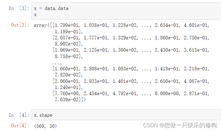
共有30个特征。

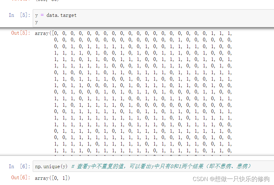
1.2 目标值

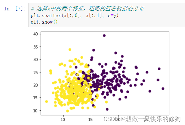
1.3 数据分布

1.3.1 选择前两维特征绘制散点图

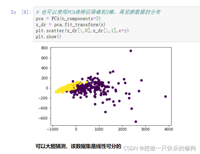
1.3.2 使用PCA降维到2维，再绘制散点图

2. 代码实现

2.1 不做数据预处理，直接选择核函数

代码；

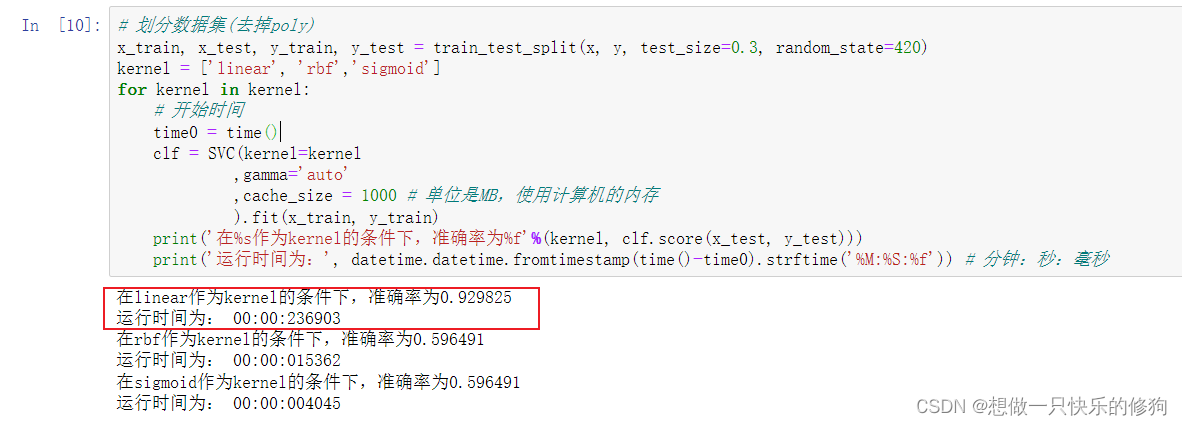
# 划分数据集
x_train, x_test, y_train, y_test = train_test_split(x, y, test_size=0.3, random_state=420)
kernel = ['linear', 'poly', 'rbf','sigmoid']
for kernel in kernel:
    # 开始时间
    time0 = time()
    clf = SVC(kernel=kernel
             ,gamma='auto'
             ,cache_size = 1000 # 单位是MB，使用计算机的内存
             ).fit(x_train, y_train)
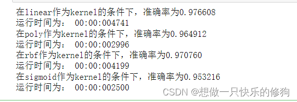
    print('在%s作为kernel的条件下，准确率为%f'%(kernel, clf.score(x_test, y_test)))
    print('运行时间为：', datetime.datetime.fromtimestamp(time()-time0).strftime('%M:%S:%f')) # 分钟：秒：毫秒

发现结果一直停在线性函数不动，因为poly作为核函数，要花费很长时间。

将poly核函数去掉，结果：

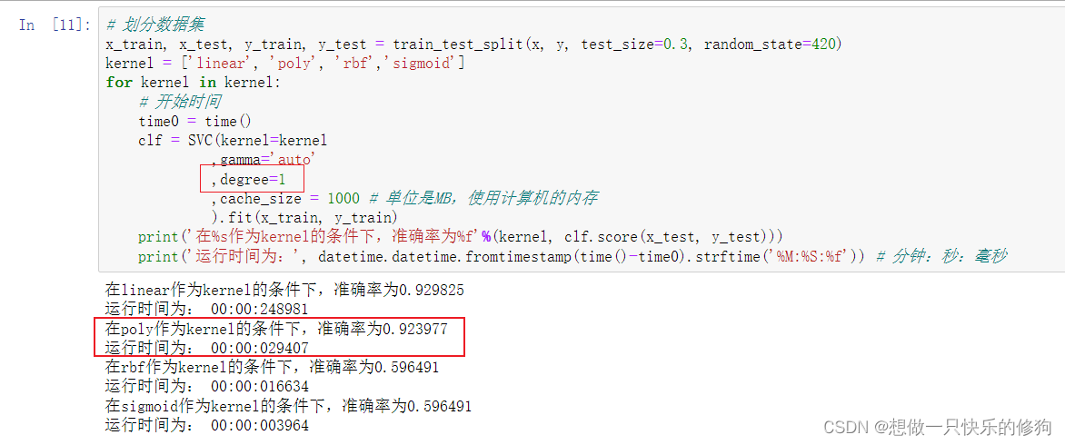
如果数据是线性的，那如果我们把degree参数调整为1，多项式核函数应该也可以得到不错的结果：

• 这样就直接选择linear了吗？可以再探索探索。

2.2 进行数据标准化，再选择核函数

2.2.1 为什么要对乳腺癌数据集进行标准化？

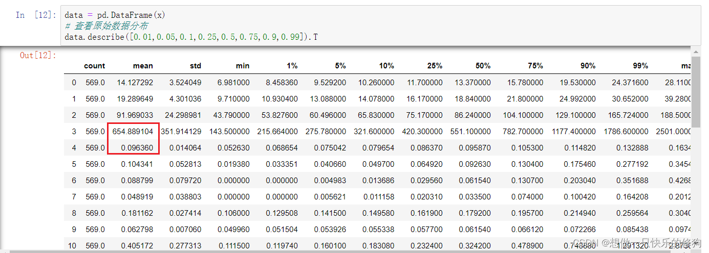
就从框出来的那个地方看，就能看出来数据量钢化差别太大，所以要进行数据标准化。
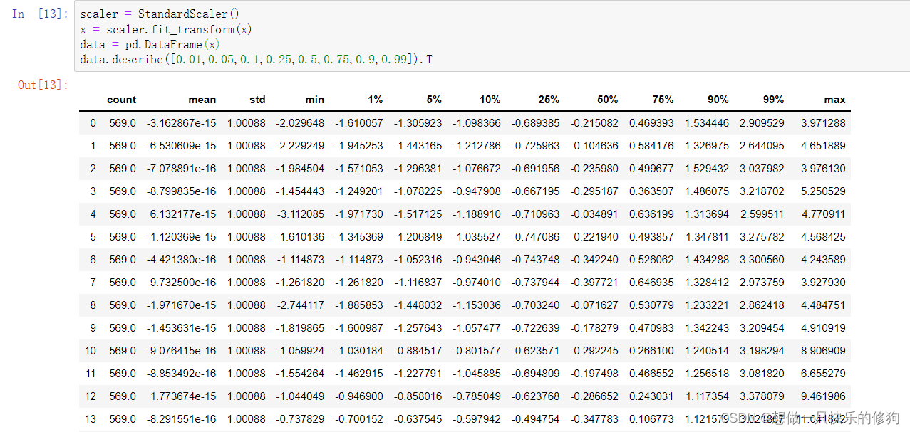
对数据进行标准化以后，再查看数据的分布：

2.2.2 代码实现

# 划分数据集(degree设置为1)
x_train, x_test, y_train, y_test = train_test_split(x, y, test_size=0.3, random_state=420)
kernel = ['linear', 'poly', 'rbf','sigmoid']
for kernel in kernel:
    # 开始时间
    time0 = time()
    clf = SVC(kernel=kernel
             ,gamma='auto'
             ,degree=1
             ,cache_size = 1000 # 单位是MB，使用计算机的内存
             ).fit(x_train, y_train)
    print('在%s作为kernel的条件下，准确率为%f'%(kernel, clf.score(x_test, y_test)))
    print('运行时间为：', datetime.datetime.fromtimestamp(time()-time0).strftime('%M:%S:%f')) # 分钟：秒：毫秒

结果：

可以见到，在rbf作为核函数的结果中精确度已经提高了，跟linear作为核函数差距没有那么大了。
那么，接下来我们就继续在rbf核函数上继续探索吧！

2.3 rbf作为核函数，继续进行调参

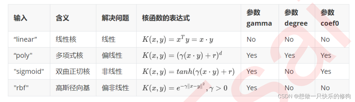
首先，看一下SVM中各个核函数所要调节的参数。

2.3.1 调节gamma —— 绘制学习曲线

score = []
gamma_range = np.logspace(-10,1,50) # 对数刻度上均匀间隔的数字
for i in gamma_range:
    clf = SVC(kernel='rbf', gamma=i, cache_size=1000).fit(x_train, y_train)
    score.append(clf.score(x_test,y_test))
    
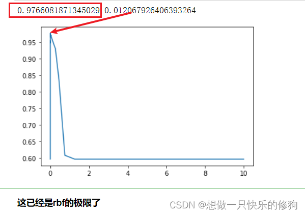
print(max(score), gamma_range[score.index(max(score))])
plt.plot(gamma_range, score)
plt.show()

结果：

2.4 kernel为poly，继续进行探索 —— 网格搜索

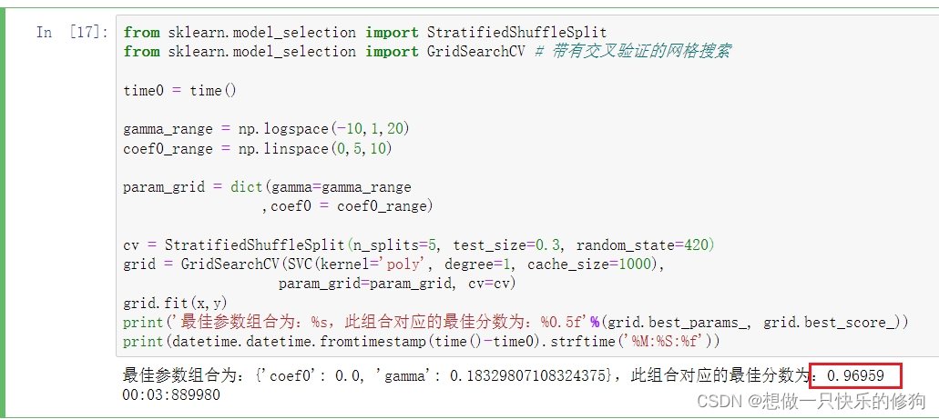
放弃poly作为核函数吧。。。

2.5 最后的挣扎，调整惩罚项系数C（linear和rbf做最后的比拼）

2.5.1 线性函数作为核函数

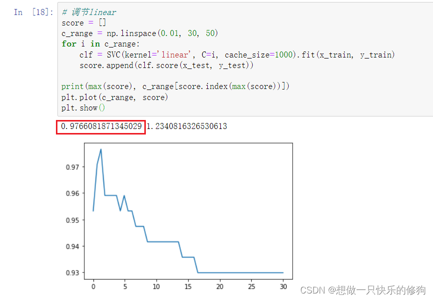
2.5.2 rbf作为核函数

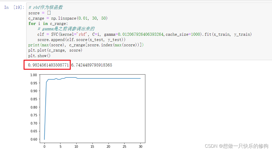
啊啊啊啊啊啊啊啊啊啊，努力没有白费啊！

结论

针对sklearn中的乳腺癌数据集，使用SVC作为算法模型，进行调参，最优的参数组合为：

核函数	gamma	惩罚项C
rbf	0.012067926406393264	6.7424489795918365

---

【PS】这是我看看sklearn菜菜的视频学习笔记~