岭回归和lasso回归_第七天：正则化，岭回归，LASSO回归和弹性网络

上一期我们讲过过拟合是机器学习中常见的问题，具体表现在虽然模型的训练误差在不断减小，但是模型的测试误差在不断增大，也就是说模型的泛化能力很差，如下图所示：

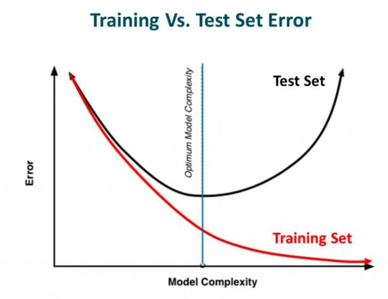
过拟合的本质是机器学习的模型过于复杂，因此学习到了训练数据中的奇异值或噪声，因此对未见过的数据识别能力很差。正则化技术能够改善模型在未知数据上的表现，提高机器学习模型的泛化能力。

根据奥卡姆剃刀原理，在所有可能选择的模型中，能很好解释已知数据，并且十分简单的模型才是最好的模型。因此，正则化就是在最小经验误差函数的基础上加上先验知识的约束(例如据奥卡姆剃刀原理中的模型越简单越好，l-norm先验中的稀疏平滑解等)。该约束可以引导机器学习模型在训练时倾向于选择满足约束的梯度下降方向，使得最终学习得到的机器学习模型鲁棒，稳定而且适定。

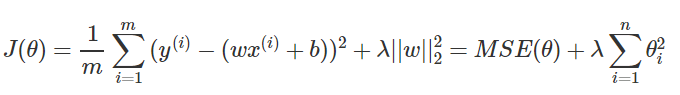
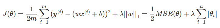
L1 和 L2 正则化是最常用的正则化方法。L1 正则化向目标函数添加L1范数正则化项，以减少参数的绝对值总和；而 L2 正则化中，添加L2范数正则化项的目的在于减少参数平方的总和。因此，L1 正则化中的很多参数向量是稀疏向量，很多参数趋近于0，常用于特征选择设置中。L1 正则化中的参数是值很小的稠密解，能够提高模型的泛化能力，所以机器学习中最常用的正则化方法是对权重施加 L2 范数约束。

(1)岭回归(L2正则化)：

(2)LASSO回归(L1正则化)：

(3)弹性网络：为L1正则化和L2正则化的混合体。

---

练习代码

1. 岭回归

import matplotlib.pyplot as pltimport numpy as npfrom sklearn import datasets, linear_model,model_selectionfrom sklearn.model_selection import cross_validatedef load_data():    diabetes = datasets.load_diabetes()#使用 scikit-learn 自带的一个糖尿病病人的数据集    return model_selection.train_test_split(diabetes.data,diabetes.target,      test_size=0.25,random_state=0) # 拆分成训练集和测试集，测试集大小为原始数据集大小的 1/4def test_Ridge(*data):    X_train,X_test,y_train,y_test=data    regr = linear_model.Ridge()    regr.fit(X_train, y_train)    print('Coefficients:%s, intercept %.2f'%(regr.coef_,regr.intercept_))    print("Residual sum of squares: %.2f"% np.mean((regr.predict(X_test) - y_test) ** 2))    print('Score: %.2f' % regr.score(X_test, y_test))def test_Ridge_alpha(*data):    X_train,X_test,y_train,y_test=data    alphas=[0.01,0.02,0.05,0.1,0.2,0.5,1,2,5,10,20,50,100,200,500,1000]    scores=[]    for i,alpha in enumerate(alphas):        regr = linear_model.Ridge(alpha=alpha)        regr.fit(X_train, y_train)        scores.append(regr.score(X_test, y_test))  ## 绘图    fig=plt.figure()    ax=fig.add_subplot(1,1,1)    ax.plot(alphas,scores)    ax.set_xlabel(r"$\alpha$")    ax.set_ylabel(r"score")    ax.set_xscale('log')    ax.set_title("Ridge")    plt.show()if __name__=='__main__':    X_train,X_test,y_train,y_test=load_data() # 产生用于回归问题的数据集test_Ridge(X_train,X_test,y_train,y_test) # 调用 test_Ridge

2. LASSO回归

import matplotlib.pyplot as pltimport numpy as npfrom sklearn import datasets, linear_model,model_selectiondef load_data():    diabetes = datasets.load_diabetes()#使用 scikit-learn 自带的一个糖尿病病人的数据集    return model_selection.train_test_split(diabetes.data,diabetes.target,      test_size=0.25,random_state=0) # 拆分成训练集和测试集，测试集大小为原始数据集大小的 1/4def test_Lasso(*data):    X_train,X_test,y_train,y_test=data    regr = linear_model.Lasso()    regr.fit(X_train, y_train)    print('Coefficients:%s, intercept %.2f'%(regr.coef_,regr.intercept_))    print("Residual sum of squares: %.2f"% np.mean((regr.predict(X_test) - y_test) ** 2))    print('Score: %.2f' % regr.score(X_test, y_test))def test_Lasso_alpha(*data):    X_train,X_test,y_train,y_test=data    alphas=[0.01,0.02,0.05,0.1,0.2,0.5,1,2,5,10,20,50,100,200,500,1000]    scores=[]    for i,alpha in enumerate(alphas):        regr = linear_model.Lasso(alpha=alpha)        regr.fit(X_train, y_train)        scores.append(regr.score(X_test, y_test))    ## 绘图    fig=plt.figure()    ax=fig.add_subplot(1,1,1)    ax.plot(alphas,scores)    ax.set_xlabel(r"$\alpha$")    ax.set_ylabel(r"score")    ax.set_xscale('log')    ax.set_title("Lasso")    plt.show()if __name__=='__main__':    X_train,X_test,y_train,y_test=load_data() # 产生用于回归问题的数据集    test_Lasso(X_train,X_test,y_train,y_test) # 调用 test_Lasso

3. 弹性网络

import matplotlib.pyplot as pltimport numpy as npfrom sklearn import datasets, linear_model,model_selectiondef load_data():    diabetes = datasets.load_diabetes()#使用 scikit-learn 自带的一个糖尿病病人的数据集    return model_selection.train_test_split(diabetes.data,diabetes.target,      test_size=0.25,random_state=0) # 拆分成训练集和测试集，测试集大小为原始数据集大小的 1/4def test_ElasticNet(*data):    X_train,X_test,y_train,y_test=data    regr = linear_model.ElasticNet()    regr.fit(X_train, y_train)    print('Coefficients:%s, intercept %.2f'%(regr.coef_,regr.intercept_))    print("Residual sum of squares: %.2f"% np.mean((regr.predict(X_test) - y_test) ** 2))    print('Score: %.2f' % regr.score(X_test, y_test))def test_ElasticNet_alpha_rho(*data):    X_train,X_test,y_train,y_test=data    alphas=np.logspace(-2,2)    rhos=np.linspace(0.01,1)    scores=[]    for alpha in alphas:            for rho in rhos:                regr = linear_model.ElasticNet(alpha=alpha,l1_ratio=rho)                regr.fit(X_train, y_train)                scores.append(regr.score(X_test, y_test))    ## 绘图    alphas, rhos = np.meshgrid(alphas, rhos)    scores=np.array(scores).reshape(alphas.shape)    from mpl_toolkits.mplot3d import Axes3D    from matplotlib import cm    fig=plt.figure()    ax=Axes3D(fig)    surf = ax.plot_surface(alphas, rhos, scores, rstride=1, cstride=1, cmap=cm.jet,        linewidth=0, antialiased=False)    fig.colorbar(surf, shrink=0.5, aspect=5)    ax.set_xlabel(r"$\alpha$")    ax.set_ylabel(r"$\rho$")    ax.set_zlabel("score")    ax.set_title("ElasticNet")    plt.show()if __name__=='__main__':    X_train,X_test,y_train,y_test=load_data() # 产生用于回归问题的数据集    test_ElasticNet(X_train,X_test,y_train,y_test) # 调用 test_ElasticNet

---

参考文献：

[1]https://mp.weixin.qq.com/s/VVHe2msyeUTGiC7f_f0FFA

[2]https://mp.weixin.qq.com/s/B9fVyN8cXFDw8BpUjIg8dg

关注“人工智能教育”公众号，您将获得我们精选的机器学习教材和代码，谢谢！