tensorflow loss到多少_RNN/LSTM/GRU 详解+tensorflow使用

• Vanilla RNN
  • RNN模型结构
  • RNN可以处理的任务
  • RNN的训练
    • backpropagation through time（BPTT）
  • RNN code demo
  • RNN的缺点
  • ref
• LSTM
  • 网络结构
  • Code Demo
  • 为什么能解决gradient vanishing
  • ref
• GRU
  • code demo
  • ref
• RNN Extension
  • Bidirectional RNN
    • code
  • Deep RNN
    • Code Demo
• difference
• tensorflow API

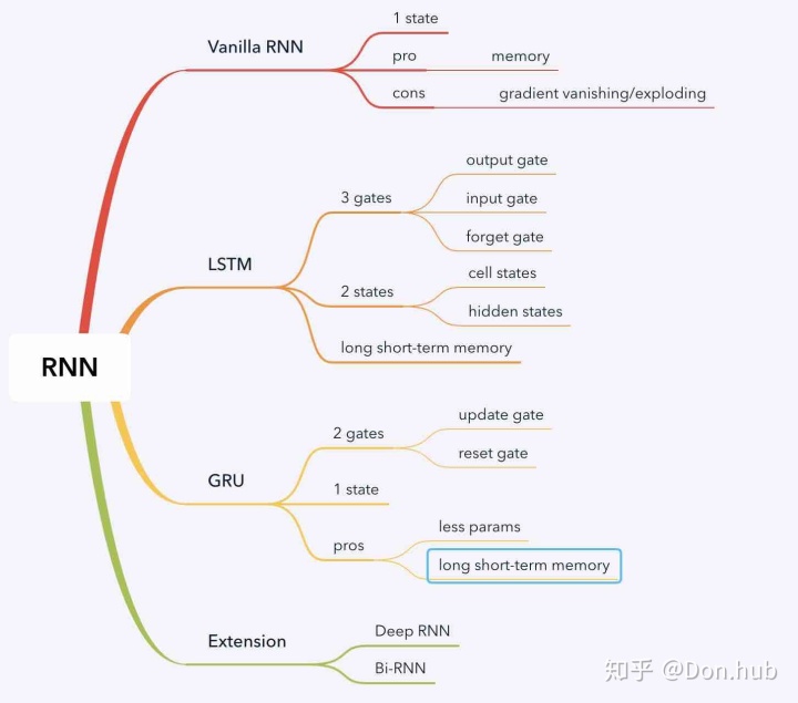
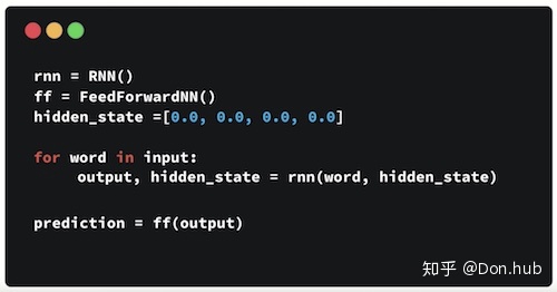
Vanilla RNN

当我们输入是一段序列的时候，传统的DNN是假设序列的token之间是互相独立的，但是在很多情况下，这是不合理的。

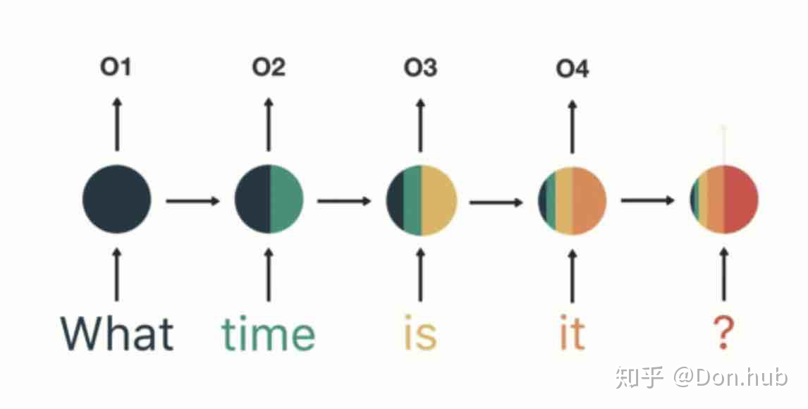
例如一个句子：

他从小生活在法国，所以他说一口流利的__。 答案法语。

我们在预测这个空的时候，我们根据这个序列之前的知识，可以非常容易地判断这个地方应该填写什么。所以我们需要一个网络，可以储存之前序列的记忆，用来作之后序列的预测。

RNN就是基于机制所发明的模型结构。其主要的作用在于能够支持Short-term Memory，然后对序列输入取得了很好的结果，但是这边我们也提出了，它支持的是短时间的memory 对于远距离的memory，RNN因为gradient vanish/explode 导致不能够支持长距离的memroy。这时候就有LSTM或者GRU来解决此类问题。

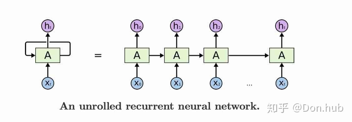
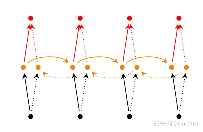
RNN模型结构

注意：bias ignored here

• : 是t时刻的输入状态
• ：element-wise元素相乘
• ： 是t时刻的隐藏状态，这个可以看作是模型的memory 的空间，它依赖的是模型当前的输入以及模型之前的hidden state。init hidden state通常是 all zeros。它捕获了之前所有的time steps的信息，但是实际上就如之前所说的，实际上，模型很难捕获长距离的信息。
• ： 激活函数，一般是tanh或者ReLU
• : t时刻的模型输出，他是根据t时刻的hidden states的输出进行预测。 注意序列间的token是一个token一个token传入到模型中的。RNN的这些参数在每个 time steps都是共享的，这体现的是在每个time step都进行相同的任务只是不同的输入而已，而且每次都更新memory。这很大地减少了参数量。 虽然每个time step都是有y的输出，但是这取决于你的任务，如果是序列标注任务需要的是所有step的输出y，但是如果是分类任务，或者编码任务，就只需要最后一个timestamp的输出。

RNN可以处理的任务

这边所讲的任务都泛指所有的RNN，包含各种变形LSTM，GRU或者结构组合Bi-RNN等。

• Text Classification RNN做文本分类
• machine translation sequence2sequence任务，中就是使用RNN的
• Language model ELMo使用的就是RNN做语言模型的预训练

RNN的训练

对于RNN的训练我们同样也是使用back propagation。但是因为我们模型的参数是共享的，当前step的输出不仅仅依赖于当前的step，而且还依赖于之前的steps，例如要计算

我们需要backpropagate 3 steps，然后再把这些gradient加和起来，这就是backpropagation through time（BPTT）。正如我们所说的，vanilla RNN在捕获长距离依赖信息有困难，我们可以看到下图，越后面time step的信息，占hidden state的比重越大，这是因为gradient vanishing/exploding的问题。

backpropagation through time（BPTT）

简单的说：在time step

时， loss

:

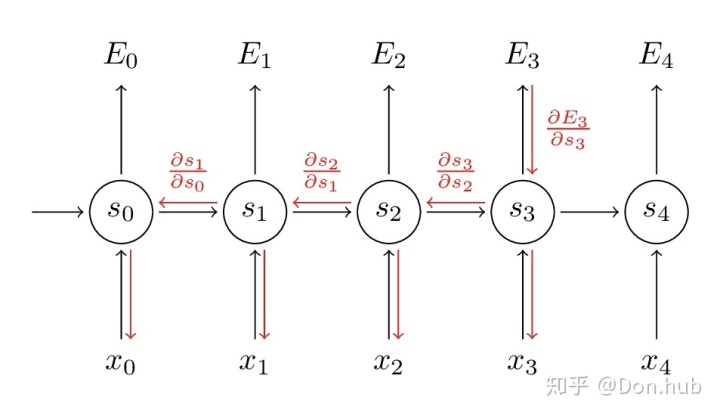
其中

因为我们使用的是tanh的函数，这个函数的gradient在value值很大的时候，为0，这时候多个连乘的时候，就会导致为0，造成gradient vanishing。或者如果多个大的梯度的时候，会出现gradient exploding。 注意这边越之前的hidden state越可能遇到这种问题，所以越后面time step的占比越大。 see ref for clear explanation.

RNN code demo

import tensorflow as tf
import numpy as np

# hyperparameters
hidden_size = 4
X_data = np.array([
# steps   1st     2nd       3rd
        [[1.0, 2], [7, 8], [13, 14]],  # first batch
        [[3, 4], [9, 10], [15, 16]], # second batch
        [[5, 6], [11, 12], [17, 18]] # third batch
]) # shape: [batch_size, n_steps, n_inputs]
# parameters
n_steps = X_data.shape[1]
n_inputs = X_data.shape[2]

# rnn model
X = tf.placeholder(tf.float32, [None, n_steps, n_inputs])

output, state = tf.nn.dynamic_rnn(tf.nn.rnn_cell.BasicRNNCell(hidden_size), X, dtype=tf.float32)
# initializer the variables
init = tf.global_variables_initializer()

# train
with tf.Session() as sess:
    sess.run(init)
    feed_dict = {X: X_data}
    output = sess.run(output, feed_dict=feed_dict)
    state = sess.run(state, feed_dict=feed_dict)
    print('output: n', output) # 所有sequence token的hidden state
    print('output shape [batch_size, n_steps, n_neurons]: ', np.shape(output))
    print('state: n', state) # 最后的hidden state
    print('state shape [n_layers, batch_size, n_neurons]: ' , np.shape(state))

--------------
output:
 [[[ 0.92815584 -0.13206302  0.5850617  -0.42844245]
  [ 0.9999997  -0.8181832   0.9910015  -0.999738  ]
  [ 1.         -0.81327766  0.99976206 -0.9999997 ]]

 [[ 0.9989392  -0.22176631  0.8764293  -0.89338243]
  [ 1.         -0.8668415   0.99713266 -0.99997586]
  [ 1.         -0.83321404  0.99993896 -1.        ]]


 [[ 0.999985   -0.3078668   0.967407   -0.9842752 ]
  [ 1.         -0.8832955   0.9991832  -0.99999714]
  [ 1.         -0.8567056   0.9999845  -1.        ]]]
output shape [batch_size, n_steps, n_neurons]:  (3, 3, 4)
state:
 [[ 1.         -0.81327766  0.99976206 -0.9999997 ]
 [ 1.         -0.83321404  0.99993896 -1.        ]
 [ 1.         -0.8567056   0.9999845  -1.        ]]
state shape [n_layers, batch_size, n_neurons]:  (3, 4)

RNN的缺点

• gradient vanishing， LSTM或者GRU解决

• 不能并行，transformer

ref

http://www.wildml.com/2015/09/recurrent-neural-networks-tutorial-part-1-introduction-to-rnns/ https://towardsdatascience.com/illustrated-guide-to-recurrent-neural-networks-79e5eb8049c9 http://www.wildml.com/2016/08/rnns-in-tensorflow-a-practical-guide-and-undocumented-features/

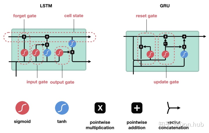
LSTM

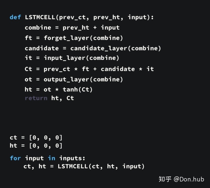
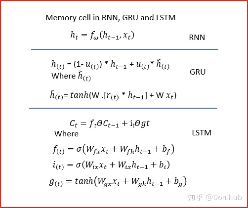
LSTM is short for Long Short-term memory。主要的作用是解决Naive RNN的训练过程中梯度消失的问题。它引入了一个cell state，这个cell state的改变比hidden state的改变更慢，因为cell state是在原本的cell state的基础上选择性更加内容，而hidden state的是直接全部更新替换。

• h 更新快，因为是直接更改的，
• c 更新慢，因为是原本的c基础上更新的，

网络结构

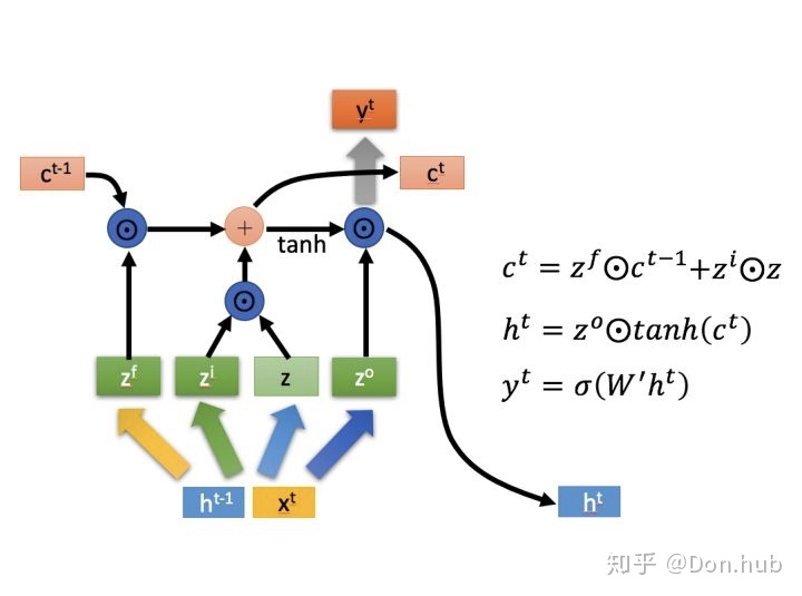
模型将

concat起来，获取三个门以及一个更新量

• ：cell state的更新量
• ：输入门，选择性记忆本时刻的输入。[选择记忆阶段]
• ：遗忘门，用来选择之前的cell state需要遗忘多少。[忘记阶段]
• ：输出门，用来选择多少的输出量可以作为最后输出。[输出阶段]
• ：element-wise元素相乘
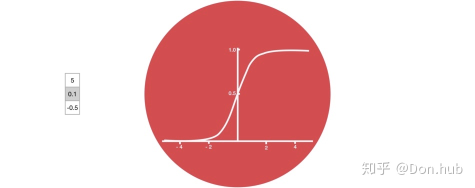
• ：sigmoid激活函数，因为它可以将数值映射为0-1区间中，0代表门关闭，1代表门打开。

在这个之后我们可以获得cell state当前时刻的输出，以及当前时刻output的输出值。

• ：我们的输出是仅仅依赖于cell state的当前输出，不经过其他的变换，再通过输出门。
• : t时刻的模型输出，他是根据t时刻的hidden states的输出进行预测。和普通的RNN一样。

Code Demo

import tensorflow as tf
import numpy as np

# batch size = 2
# sequence_length = 10
# embedding dim = 8
X = np.random.randn(2, 10, 8)
hidden_size = 4
# make the second example, padding for sequence > 6, which means that the second example has length 6
X[1,6:] = 0

# specify the length for each example, first is 10, second is 6
#you tell Tensorflow to stop calculations for example 2 at step 6
# and simply copy the state from time step 6 to the end.
X_lengths = [10, 6] # batch 中的sequence的长度, 可以指定我们的每个sequence的长度！！

cell = tf.nn.rnn_cell.LSTMCell(num_units=hidden_size, state_is_tuple=True)
"""
Internally, tf.nn.rnn creates an unrolled graph for a fixed RNN length. That means, if you call tf.nn.rnn with inputs having 200 time steps you are creating a static graph with 200 RNN steps. First, graph creation is slow. Second, you’re unable to pass in longer sequences (> 200) than you’ve originally specified.

tf.nn.dynamic_rnn solves this. It uses a tf.While loop to dynamically construct the graph when it is executed. That means graph creation is faster and you can feed batches of variable size. What about performance? You may think the static rnn is faster than its dynamic counterpart because it pre-builds the graph. In my experience that’s not the case.

In short, just use tf.nn.dynamic_rnn. There is no benefit to tf.nn.rnn and I wouldn’t be surprised if it was deprecated in the future.
"""
# if you dont set sequence_length, you will get answer wrong
"""
last_states: 包含最后一层的c和h
outputs: 是每个step的hidden output [:,-1,:]就是last hidden state
"""
outputs , last_states = tf.nn.dynamic_rnn(cell=cell, dtype=tf.float64, sequence_length=X_lengths, inputs=X)
init_op = tf.global_variables_initializer()
with tf.Session() as sess:
    sess.run(init_op)
    outputs, last_states = sess.run([outputs, last_states])
    print(outputs)
    print("output's shape", np.shape(outputs)) # batch size * sequence length * hidden_size
    print(np.shape(outputs))
    print(last_states)
    print(np.shape(last_states)) # # batch size * 2 *num_units，包含了h和c的最后状态。
-----------------
[[[ 0.07664019 -0.16831291  0.13080093 -0.06008256]
  [ 0.11326599 -0.1056436  -0.08374735 -0.0958832 ]
  [ 0.08136585 -0.15087794  0.1383943  -0.05682314]
  [ 0.17250682 -0.0577739   0.20614527 -0.09149361]
  [ 0.11158117  0.03405583  0.05773997  0.00920278]
  [ 0.11854824 -0.10070093 -0.00953649 -0.10144152]
  [ 0.05768328 -0.0627834  -0.16341334 -0.18205421]

  [-0.05942476  0.2136804  -0.27391385 -0.06917706]
  [-0.41610618  0.16935246 -0.07550309 -0.11293897]
  [ 0.02186674  0.27126661  0.1722617   0.08577567]]

 [[ 0.11671963 -0.0168591   0.29560884 -0.09077734]
  [ 0.0679137   0.03817917  0.2389287  -0.06904289]
  [ 0.13058297  0.16488049  0.31145256 -0.08429188]
  [-0.15175866  0.2183992   0.29114083 -0.11348455]
  [-0.037971    0.0290376   0.17756673 -0.08450237]
  [-0.02581448 -0.11466457  0.14280298 -0.43767932]
  [ 0.          0.          0.          0.        ]
  [ 0.          0.          0.          0.        ]
  [ 0.          0.          0.          0.        ]
  [ 0.          0.          0.          0.        ]]]
output's shape (2, 10, 4)
(2, 10, 4)
LSTMStateTuple(c=array([[ 0.05822175,  0.55288346,  0.21132719,  0.21992871],
       [-0.45828684, -0.16487249,  0.43235717, -0.56931392]]), h=array([[ 0.02186674,  0.27126661,  0.1722617 ,  0.08577567],
       [-0.02581448, -0.11466457,  0.14280298, -0.43767932]]))
(2, 2, 4)

为什么能解决gradient vanishing

模型引入了cell state，cell state可以作为模型的记忆中心，他可以储存模型的很早time step的输出，减少了short term memory的影响。之前time step的信息是通过不同的门控来进行cell state的记忆或者遗忘。

在一般的RNN中，每个时刻neuron的output都会被放到memory中去，所以在每个时刻memory中的值都会被洗掉。但在LSTM中，是把memory中原来的值乘上一个数再加上一个数，即memory和input是想加的关系。所以LSTM中如果weight影响了memory中的值，那么这个影响会永远都存在（除非forget gate决定洗掉memory，有说法认为要给forget gate很大的bias以使其多数情况下开启），而不像SimpleRNN中memory的值在每个时刻都会被洗掉。 若使用LSTM出现了过拟合，可考虑改用GRU。GRU的精神是“旧的不去，新的不来”，它将input gate与forget gate联动起来：若input gate 开，则forget gate 关。

• 传统的RNN总是用“覆写”的方式计算状态：
  ，根据求导的链式法则，这种形式直接导致梯度被表示为连成积的形式，以致于造成梯度消失——粗略的说，很多个小于1的项连乘就很快的逼近零。
• 现代的RNN（包括但不限于使用LSTM单元的RNN）使用“累加”的形式计算状态：
  ，稍加推导即可发现，这种累加形式导致导数也是累加形式，因此避免了梯度消失。
• 我们之前分析RNN产生梯度消失或者梯度爆炸的原因在于
  , 令这个
  但是LSTM中

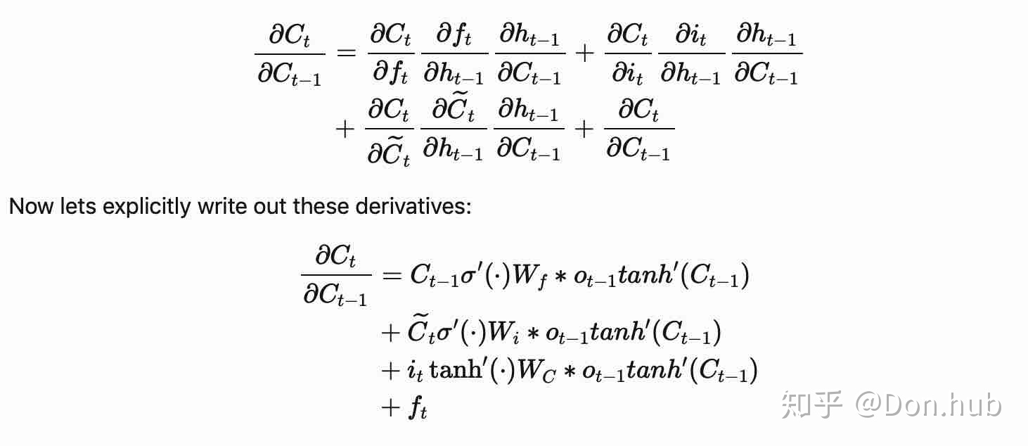
如果这个梯度要变成0了，那么将forget gate的值设为1，那么就可以减轻gradient descent的可能。通过这些门的设置可以设置让什么time step的值vanish，什么time step的值keep。

see great explanation

ref

https://zhuanlan.zhihu.com/p/32085405 https://colah.github.io/posts/2015-08-Understanding-LSTMs/ https://blog.csdn.net/xzy_thu/article/details/74930482 https://www.zhihu.com/question/34878706 https://www.cnblogs.com/bonelee/p/10475453.html http://www.wildml.com/2016/08/rnns-in-tensorflow-a-practical-guide-and-undocumented-features/ https://weberna.github.io/blog/2017/11/15/LSTM-Vanishing-Gradients.html

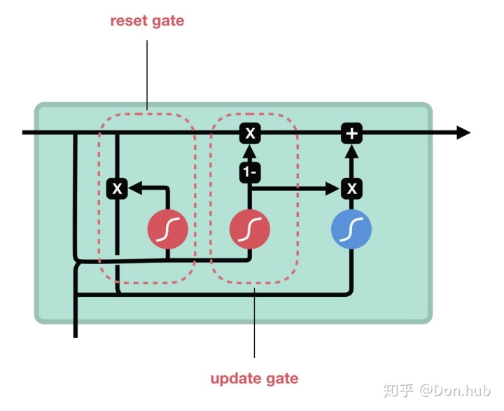
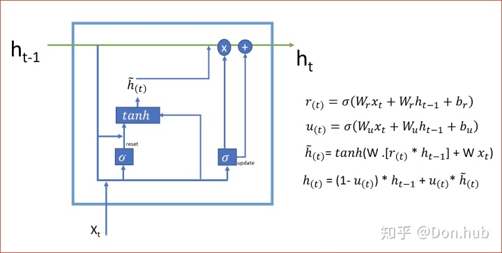
GRU

GRU是在LSTM的基础上，做的改进，在效果相近的情况下，大大减少了运算量。GRU的精神是“旧的不去，新的不来”，它将input gate与forget gate联动起来：若input gate 开，则forget gate 关。这个情况下，GRU只使用了两个门控，分别是更新门(update gate) u，和重置门(reset gate) r。

• ：为sigmoid函数
• 其中reset gate 用来重置之前的hidden state
• update gate用来选择性遗忘之前hidden state的信息和记忆新的输入更新量

替代了更新量LSTM 的更新量z，这边其实是想通的和LSTM的c的更新公式几乎一样，其中的输入更新量用的是h‘。

code demo

GRU 的使用和 Vanilla RNN一样，都只有一个中间hidden state

import tensorflow as tf
import numpy as np

# hyperparameters
hidden_size = 4
X_data = np.array([
    # steps   1st     2nd       3rd
        [[1.0, 2], [7, 8], [13, 14]],  # first batch
        [[3, 4], [9, 10], [15, 16]], # second batch
        [[5, 6], [11, 12], [17, 18]] # third batch
]) # shape: [batch_size, n_steps, n_inputs]
# parameters
n_steps = X_data.shape[1]
n_inputs = X_data.shape[2]

# rnn model
X = tf.placeholder(tf.float32, [None, n_steps, n_inputs])

output, state = tf.nn.dynamic_rnn(tf.nn.rnn_cell.GRUCell(hidden_size), X, dtype=tf.float32)
# initializer the variables
init = tf.global_variables_initializer()

# train
with tf.Session() as sess:
    sess.run(init)
    feed_dict = {X: X_data}
    output = sess.run(output, feed_dict=feed_dict)
    state = sess.run(state, feed_dict=feed_dict)
    print('output: n', output) # 所有sequence token的hidden state
    print('output shape [batch_size, n_steps, n_neurons]: ', np.shape(output))
    print('state: n', state) # 最后的hidden state
    print('state shape [n_layers, batch_size, n_neurons]: ' , np.shape(state))
'''
output:
 [[[-0.25309005 -0.14193957 -0.02487047  0.17022096]
  [-0.38218772 -0.16599673 -0.0156059   0.98334306]

  [-0.42112508 -0.16815719 -0.01516359  0.9999074 ]]

 [[-0.2583678  -0.0987941   0.01887107  0.67746955]
  [-0.34110394 -0.109093    0.02178543  0.99754757]
  [-0.3752105  -0.11028701  0.021943    0.9999824 ]]

 [[-0.23161995 -0.0572155   0.01641296  0.9205886 ]
  [-0.29479396 -0.06217026  0.0174125   0.999571  ]
  [-0.32523265 -0.06282293  0.01747114  0.9999964 ]]]
output shape [batch_size, n_steps, n_neurons]:  (3, 3, 4)
state:
 [[-0.42112508 -0.16815719 -0.01516359  0.9999074 ]
 [-0.3752105  -0.11028701  0.021943    0.9999824 ]
 [-0.32523265 -0.06282293  0.01747114  0.9999964 ]]
state shape [n_layers, batch_size, n_neurons]:  (3, 4)
'''

ref

https://iamtrask.github.io/2015/11/15/anyone-can-code-lstm/ https://zhuanlan.zhihu.com/p/32481747 https://towardsdatascience.com/illustrated-guide-to-lstms-and-gru-s-a-step-by-step-explanation-44e9eb85bf21 https://medium.com/datadriveninvestor/multivariate-time-series-using-gated-recurrent-unit-gru-1039099e545a https://towardsdatascience.com/gate-recurrent-units-explained-using-matrices-part-1-3c781469fc18 https://zh.d2l.ai/chapter_recurrent-neural-networks/gru.html http://www.wildml.com/2016/08/rnns-in-tensorflow-a-practical-guide-and-undocumented-features/

RNN Extension

Bidirectional RNN

双向的RNN指的是同一个序列，同时需用了前向的RNN以及反向的RNN进行训练，最后获得的输出是两个RNN各自的输出。

例如我们要翻译一个句子，我们不仅依赖于之前的context还依赖之后的context，使用双向的RNN可以得到更好的结构。

code

import tensorflow as tf
import numpy as np

X = np.random.randn(2, 5, 8)
hidden_size = 3
X[1, 3:] = 0
X_lengths = [5, 3]

cell = tf.nn.rnn_cell.LSTMCell(num_units=hidden_size, state_is_tuple=True)

outputs, states = tf.nn.bidirectional_dynamic_rnn(cell_fw=cell, cell_bw=cell, inputs=X, sequence_length=X_lengths, dtype=tf.float64)

output_fw, output_bw = outputs # fw output and bw output, each one is of shape [batch_size, sequence_length(time steps), num_units]
states_fw, states_bw = states # states_fw, states_bw, each one is of shape [batch_size, 2, num_units]

with tf.Session() as sess:
    sess.run(tf.global_variables_initializer())
    print(sess.run([output_fw, output_bw, states_fw, states_bw]))
    print(sess.run([tf.shape(output_fw), tf.shape(output_bw), tf.shape(states_fw), tf.shape(states_bw)]))
'''
[array([[[-0.20675935, -0.05998449, -0.11168052],
        [-0.22264413, -0.14726669, -0.36435551],
        [-0.16212785, -0.15073723, -0.50727016],
        [-0.14148236, -0.25463935, -0.50446747],
        [-0.07956968, -0.25852016, -0.603786  ]],

       [[ 0.07491359,  0.16615575,  0.04055494],
        [ 0.36352407, -0.02417577,  0.04969817],
        [ 0.07610515,  0.05123368,  0.0073431 ],
        [ 0.        ,  0.        ,  0.        ],
        [ 0.        ,  0.        ,  0.        ]]]),
array([[[-0.31525074, -0.26519498, -0.28104269],
        [-0.16510516, -0.19432073, -0.50337067],
        [-0.09027677, -0.13906253, -0.40863558],
        [ 0.11484543, -0.17231788, -0.15510134],
        [ 0.05491017, -0.06551549, -0.22044168]],
       [[ 0.1766555 ,  0.1300383 ,  0.03363542],
        [ 0.23138083, -0.0307284 , -0.01062863],
        [-0.12122436,  0.08837643, -0.04304867],
        [ 0.        ,  0.        ,  0.        ],
        [ 0.        ,  0.        ,  0.        ]]]),
LSTMStateTuple(
    c=array([[-0.13106013, -0.96111252, -1.10753714],
       [ 0.19322541,  0.11261105,  0.01296239]]),
    h=array([[-0.07956968, -0.25852016, -0.603786  ],
       [ 0.07610515,  0.05123368,  0.0073431 ]])),
LSTMStateTuple(
    c=array([[-0.77197357, -0.99756858, -1.12553549],
       [ 0.65078194,  0.20281566,  0.11306533]]),
    h=array([[-0.31525074, -0.26519498, -0.28104269],
       [ 0.1766555 ,  0.1300383 ,  0.03363542]]))]
[array([2, 5, 3], dtype=int32), array([2, 5, 3], dtype=int32), array([2, 2, 3], dtype=int32), array([2, 2, 3], dtype=int32)]
'''

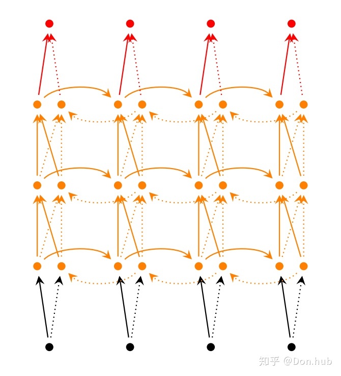
Deep RNN

RNN层可以经过多层级连，就有点类似DNN网络，前一层的hidden output作为下一层的输入。每一个time step都有多层layers，可以使得模型有更强的表达空间。

Code Demo

import tensorflow as tf
import numpy as np

# hyperparameters
n_neurons = 5
X_data = np.array([
# steps   1st     2nd       3rd
        [[1.0, 2], [7, 8], [13, 14]],  # first batch
        [[3, 4], [9, 10], [15, 16]], # second batch
        [[5, 6], [11, 12], [17, 18]] # third batch
]) # shape: [batch_size, n_steps, n_inputs]
# parameters
n_steps = X_data.shape[1]
n_inputs = X_data.shape[2]
n_layers = 6 # 5 hidden layers

# rnn model
X = tf.placeholder(tf.float32, [None, n_steps, n_inputs])
"""
Basically, to elaborate the answer from this issue:
Using [cell]*num_layers will create a list of
two references to the same cell instance but not two separate instances.
The correct behavior is that the LSTM cell at first layer should have weight shape like
(dimensionality_of_feature + cell_state_size, 4*cell_state_size).
And the LSTM cells at consecutive layers should have weight shape
like (2*cell_state_size, 4*cell_state_size).
Because they no longer take original input but the input from the previous layer.

But the problem in the shared reference code is
that for both layers they will use the same kernel
due to "they" are actually the same cell instance.
Therefore, even if you have more than one layers,
all layers except the first one will have the
wrong shape of weight (always referring to the weight of the first layer).

A better code as indicated in this issue is using
list comprehension or for loop to create multiple separate
instances to avoid sharing references.
# # cause bug
# cell = tf.nn.rnn_cell.LSTMCell(num_units=n_neurons)
# layers = [ cell for _ in range(n_layers)]
https://github.com/tensorflow/tensorflow/issues/16186
"""
def selfdefined_rnn_cell():
   lstm = tf.nn.rnn_cell.LSTMCell(n_neurons, forget_bias=1.0)
   cell = tf.nn.rnn_cell.DropoutWrapper(cell=lstm, output_keep_prob=0.5)
   return cell
multi_rnn = tf.nn.rnn_cell.MultiRNNCell([selfdefined_rnn_cell() for _ in range(n_layers)])
output, state = tf.nn.dynamic_rnn(multi_rnn, X, dtype=tf.float32)
# initializer the variables
init = tf.global_variables_initializer()

# train
with tf.Session() as sess:
    sess.run(init)
    feed_dict = {X: X_data}
    output_shape = sess.run(tf.shape(output), feed_dict=feed_dict)
    state_shape = sess.run(tf.shape(state), feed_dict=feed_dict)
    print('output shape [batch_size, n_steps, n_neurons]: ', output_shape)
    print('state shape [n_layers, batch_size, n_neurons]: ' ,state_shape)

difference

Todo: https://medium.com/datadriveninvestor/multivariate-time-series-using-gated-recurrent-unit-gru-1039099e545a

tensorflow API

基础的RNN 以及相关wrapper模块为：

• BasicRNNCell() – A vanilla RNN cell.
• GRUCell() – A Gated Recurrent Unit cell.
• BasicLSTMCell() – An LSTM cell based on Recurrent Neural Network Regularization. No peephole connection or cell clipping.
• LSTMCell() – A more complex LSTM cell that allows for optional peephole connections and cell clipping.
• MultiRNNCell() – A wrapper to combine multiple cells into a multi-layer cell.
• DropoutWrapper() – A wrapper to add dropout to input and/or output connections of a cell. and the contributed RNN cells and wrappers:
• CoupledInputForgetGateLSTMCell() – An extended LSTMCell that has coupled input and forget gates based on LSTM: A Search Space Odyssey.
• TimeFreqLSTMCell() – Time-Frequency LSTM cell based on Modeling Time-Frequency Patterns with LSTM vs. Convolutional Architectures for LVCSR Tasks
• GridLSTMCell() – The cell from Grid Long Short-Term Memory.
• AttentionCellWrapper() – Adds attention to an existing RNN cell, based on Long Short-Term Memory-Networks for Machine Reading.
• LSTMBlockCell() – A faster version of the basic LSTM cell (Note: this one is in lstm_ops.py)
• tf.nn.rnn():包装RNNcell 的模型容器，生成静态图，在模型定义的时候就已经生成了固定长度的RNN图，这意味这如果你的input有200哥time steps，那么你的图不能pass超过200长度的sequence。而且构造图的时候会比较慢。
• tf.nn.dynamic_rnn()： 包装RNNcell 的模型容器。在执行的时候，使用 tf.While loop 动态地构造RNN图，这意味这图的构建更快，并且你可以喂进去不同长度的sequence。实际上，dynamic rnn比static rnn在实践中更快速，所以推荐使用dynamic rnn。
• tf.nn.bidirectional_dynamic_rnn(): 双向RNN