


 本文介绍如何使用一维卷积神经网络(1DCNN)对UCI-HAR数据集进行人类活动识别,并探讨了模型调参的方法,包括数据标准化、滤波器数量及kernel大小的影响。
【时间序列预测/分类】 全系列60篇由浅入深的博文汇总:传送门
在熟悉了时间序列分类任务的数据分析、数据可视化、问题建模、模型评估等流程之后,本文介绍如何使用CNN模型实现人类活动识别分类任务。主要内容为:
- 如何加载和处理UCI-HAR数据集,以及如何开发1D CNN模型,达到良好的分类效果。
- 如何进一步调整模型的性能,包括数据转换,滤波器和kernel大小。
- 如何开发的 Multi-head 1D CNN模型。看下图就明白了:
代码环境:
- python 3.7.6
- tensorflow 2.1.0
- keras 2.3.1
代码在 jupyter notebook编写。完整代码部分对比较难理解的地方做了注释,稍微有点基础的,应该很容易理解。
文章目录
1. 用于活动识别的CNN模型
本文使用UCI-HAR数据集,开发一维卷积神经网络模型(1D CNN),实现多分类任务。CNN模型是针对图像分类问题而开发的,其中该模型在特征学习的过程中学习二维输入的内部表示。尽管称为一维CNN模型,但它支持多维输入作为单独的通道,类似图像的颜色通道(红色,绿色和蓝色)。一维CNN模型可以对一维数据序列进行相同的处理,例如处理多维传感器数据序列。该模型从观测序列中提取特征,将内部特征映射到不同的活动类型。
使用CNN进行序列分类的好处是,可以直接从原始时间序列数据中学习,专业的信号处理和特征工程相关知识。该模型可以学习时间序列数据的内部表示,理想情况下可以达到与在经过特征工程的数据集上传统机器学习方法相近的性能。
1.1 数据加载
这部分在之前的文章中已经详细地介绍过了,此处不再赘述。代码在完整代码中给出。
之前的文章:👉传送门。
1.2 建模分析
现在已将数据加载到内存中,接下来,定义可以定义,拟合和评估一维CNN模型。定义一个 evaluate_model() 函数,该函数接受训练和测试数据集,在训练数据集上拟合模型,在测试数据集上对其进行评估,然后返回模型性能的估算值。使用Keras深度学习库定义CNN模型,该模型要求输入的shape为: [样本,时间步长,特征] ([samples, timesteps, features]) 的三维输入。
这就是我们加载数据的方式,其中一个样本是时间序列数据的一个窗口,每个窗口有128个时间步长,而一个时间步长有9个变量(特征)。该模型的输出将是一个六元素向量,其中包含给定窗口属于六种活动类型中的每一种的概率。拟合模型需要这些输入和输出尺寸,可以从训练数据集中提取,代码如下:
n_timesteps, n_features, n_outputs = trainX.shape[1], trainX.shape[2], trainy.shape[1]
乍一看可能有些疑惑,看一下数据的shape就一目了然了:
trainX.shape:(7352, 128, 9),trainy.shape:(7352, 1)
testX.shape:(2947, 128, 9),testy.shape:(2947, 1)
将模型定义为顺序模型结构,有两个1D CNN层,然后是用于规范化的dropout层,然后是池化层。通常,以两个为一组来定义CNN层,以便使模型有很好的机会从输入数据中学习特征。 CNN的学习速度非常快,因此Dropout层旨在帮助减慢学习过程,降低过拟合风险,有助于提高模型泛化能力。池化层将学习到的特征降采样到原大小的四分之一。在卷积层和池化层之后,通过Flatten层将学习到的特征展平为一个长向量,之后是全连接层,然后再用输出层进行预测。理想情况下,全连接层在学习的特征和输出之间提供缓冲区,目的是在进行预测之前解释学习的特征。
对于此模型,使用64个并行特征图(64个filters)的标准配置,kernel大小为3。特征图是输入被处理或解释的次数,而kernel大小可认为是输入时间步长的长度。输入序列被读取或处理到特征图上。对于多类分类任务,将、使用随机梯度下降算法Adam来优化网络,并、使用分类交叉熵损失函数。
模型定义如下:
model = Sequential()
model.add(Conv1D(filters=64, kernel_size=3, activation='relu',input_shape=(n_timesteps,n_features)))
model.add(Conv1D(filters=64, kernel_size=3, activation='relu'))
model.add(Dropout(0.5))
model.add(MaxPooling1D(pool_size=2))
model.add(Flatten())
model.add(Dense(100, activation='relu'))
model.add(Dense(n_outputs, activation='softmax'))
model.compile(loss='categorical_crossentropy', optimizer='adam', metrics=['accuracy'])
该模型适合固定数量的epoch,在这种情况下为10个。批次大小为32,在更新模型权重之前,将32个数据窗口输入模型。模型拟合后,在测试数据集上对其进行评估,并返回测试数据集上的拟合模型的准确性。
1.3 完整代码
import pandas as pd
import numpy as np
import matplotlib.pyplot as plt
import os

from tensorflow.keras.models import Sequential
from tensorflow.keras.layers import Dense, Flatten, Dropout
from tensorflow.keras.layers import Conv1D, MaxPooling1D
from tensorflow.keras.utils import to_categorical

def load_file(filepath):
    dataframe = pd.read_csv(filepath, header=None, delim_whitespace=True)
    return dataframe.values

def load_dataset(data_rootdir, dirname, group):
    '''
    该函数实现将训练数据或测试数据文件列表堆叠为三维数组
    '''
    filename_list = []
    filepath_list = []
    X = []

    # os.walk() 方法是一个简单易用的文件、目录遍历器,可以高效的处理文件、目录。
    for rootdir, dirnames, filenames in os.walk(data_rootdir + dirname):
        for filename in filenames:
            filename_list.append(filename)
            filepath_list.append(os.path.join(rootdir, filename))
        #print(filename_list)
        #print(filepath_list)

    # 遍历根目录下的文件,并读取为DataFrame格式;
    for filepath in filepath_list:
        X.append(load_file(filepath))

    X = np.dstack(X) # dstack沿第三个维度叠加,两个二维数组叠加后,前两个维度尺寸不变,第三个维度增加;
    y = load_file(data_rootdir+'/y_'+group+'.txt')
    print('{}_X.shape:{},{}_y.shape:{}\n'.format(group,X.shape,group,y.shape))
    return X, y

def evaluate_model(trainX, trainy, testX, testy):
    verbose, epochs, batch_size = 0, 10, 32
    n_timesteps, n_features, n_outputs = trainX.shape[1], trainX.shape[2], trainy.shape[1]
    model = Sequential()
    model.add(Conv1D(filters=64, kernel_size=3, activation='relu', input_shape=(n_timesteps,n_features)))
    model.add(Conv1D(filters=64, kernel_size=3, activation='relu'))
    model.add(Dropout(0.5))
    model.add(MaxPooling1D(pool_size=2))
    model.add(Flatten())
    model.add(Dense(100, activation='relu'))
    model.add(Dense(n_outputs, activation='softmax'))
    model.compile(loss='categorical_crossentropy', optimizer='adam', metrics=['accuracy'])

    model.fit(trainX, trainy, epochs=epochs, batch_size=batch_size, verbose=verbose)

    _, accuracy = model.evaluate(testX, testy, batch_size=batch_size, verbose=0)

    return accuracy

def run_experiment(trainX, trainy, testX, testy, repeats=10):
    # one-hot编码
    # 这个之前的文章中提到了,因为原数据集标签从1开始,而one-hot编码从0开始,所以要先减去1
    trainy = to_categorical(trainy-1)
    testy = to_categorical(testy-1)

    scores = []
    for r in range(repeats):
        score = evaluate_model(trainX, trainy, testX, testy)
        score = score * 100.0
        print('>#%d: %.3f' % (r+1, score))
        scores.append(score)
        print(scores)

    mean_scores, std_scores = np.mean(scores), np.std(scores)
    print('Accuracy: %.3f%% (+/-%.3f)' % (mean_scores, std_scores))

train_dir = 'D:/GraduationCode/01 Datasets/UCI HAR Dataset/train/'
test_dir = 'D:/GraduationCode/01 Datasets/UCI HAR Dataset/test/'
dirname = '/Inertial Signals/'
trainX, trainy = load_dataset(train_dir, dirname, 'train')
testX, testy = load_dataset(test_dir, dirname, 'test')
run_experiment(trainX, trainy, testX, testy, repeats=1)
输出结果:
train_X.shape:(7352, 128, 9),train_y.shape:(7352, 1)

test_X.shape:(2947, 128, 9),test_y.shape:(2947, 1)

>#1: 91.788
[91.78826212882996]
Accuracy: 91.788% (+/-0.000)
2. 调参
2.1 数据
处理
在上一节中,直接使用数据集中处理好的样本进行训练,没有做任何处理。每个主要数据集(人体加速度,人体陀螺仪和总加速度)已缩放到[-1,1]。改进的一种可能变换是在拟合模型之前对其进行标准化。
标准化是转换变量的分布,使其平均值为零,标准偏差为1。这仅在每个变量的分布都为高斯分布时才有意义。可以通过在训练数据集中绘制每个变量的直方图来快速检查每个变量的分布。这样做的一个小困难是,数据已被分成128个时间步长窗口宽度的样本,并且是有50%重叠的采样。因此,为了对数据分布有一个清晰的了解,必须先删除重复的观测值(每个样本中的重叠部分数据)。
可以使用numpy数组切片实现,仅保留每个窗口的后半部分,然后将每个变量的窗口平展为一个长向量。去重处理和绘制分布直方图在上篇文章中讲过,代码实现如下:
cut = int(trainX.shape[1] / 2) # 去重
longX = trainX[:, -cut:, :] # 切片截取
longX = longX.reshape((longX.shape[0] * longX.shape[1], longX.shape[2])) # 将窗口数据展平
完整代码:
def plot_variable_histograms(data):
    '''
    该函数实现绘制训练集直方图;
    '''
    # 去重
    cut = int(data.shape[1] / 2)
    longX = data[:, -cut:, :]
    longX = longX.reshape((longX.shape[0] * longX.shape[1], longX.shape[2]))
    print('longX.shape:', longX.shape)
    # 绘图
    plt.figure(figsize=(12,20), dpi=150)

    name_list = ['total acc ', 'body acc ', 'body gyro ']
    axis_list = ['x', 'y', 'z']
    features_list = []
    for name in name_list:
        for axis in axis_list:
            features_list.append(name+axis)

    for i in range(len(features_list)):
        ax = plt.subplot(longX.shape[1], 1, i+1)
        ax.set_xlim(-1, 1)
        ax.hist(longX[:, i], bins=100, density=True, histtype='bar', stacked=True)
        plt.title(features_list[i], y=0, loc='left', size=18)

    plt.ylabel(r'$Value$', size=16)
    plt.xlabel(r'$timesteps$', size=16)
    plt.tight_layout()
    plt.show()

plot_variable_histograms(trainX)
运行示例将训练数据集中的九个特征的直方图。绘图顺序与数据集中顺序保持一致。
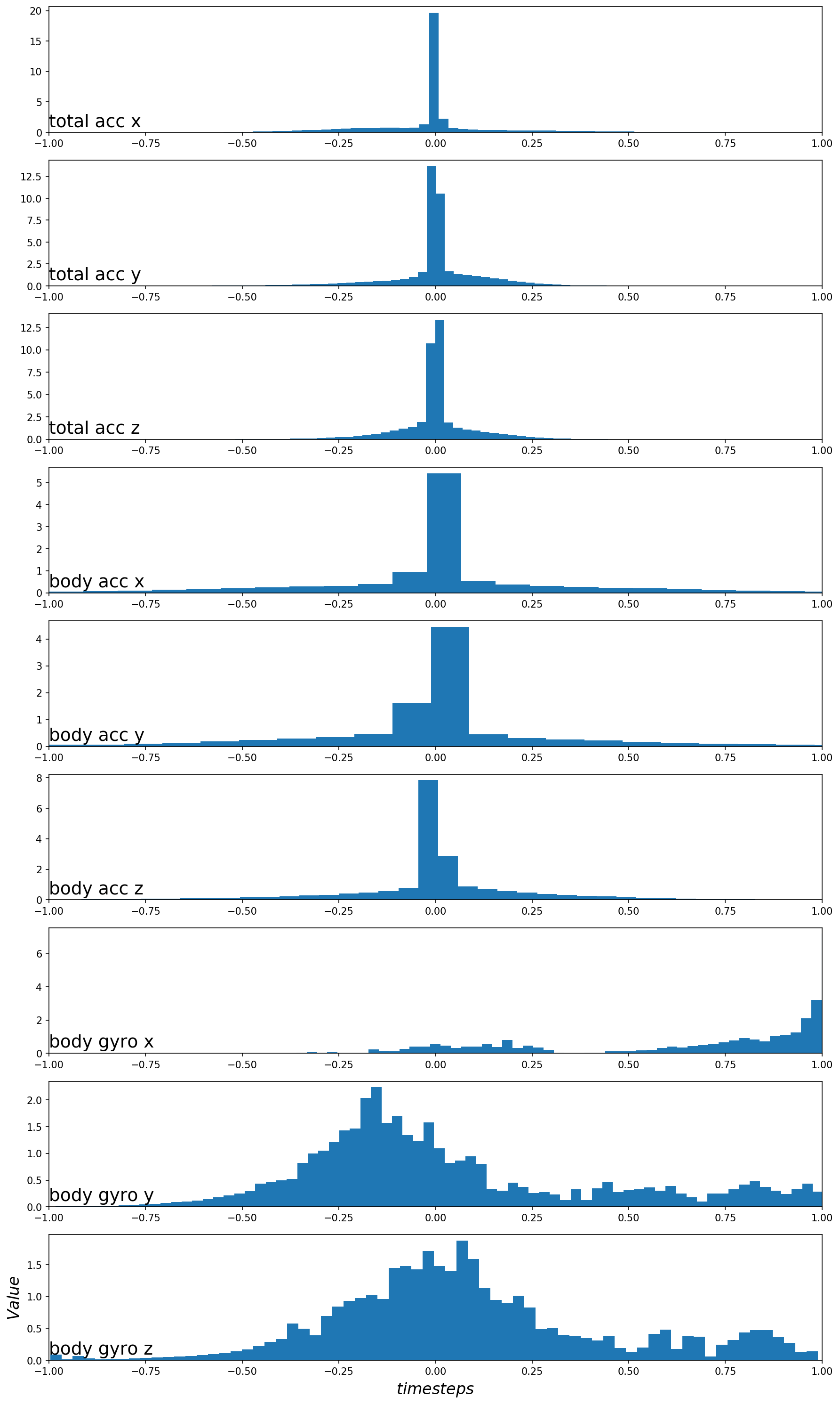
2.2 数据标准化的影响
数据具有高斯性质,探索标准化变换是否将有助于模型从原始观测值中提取显著信号。自定义一个函数实现在拟合和评估模型之前标准化数据。 可以使用scikit-learn中的StandardScaler类实现。它首先拟合训练数据(例如找到每个变量的均值和标准差),然后应用于训练和测试集。标准化是可选的,可以对比有标准化和无标准化处理的数据在模型表现上的差异。代码实现:
from sklearn.preprocessing import StandardScaler
import pandas as pd
import numpy as np
import matplotlib.pyplot as plt
import os

from tensorflow.keras.models import Sequential
from tensorflow.keras.layers import Dense, Flatten, Dropout
from tensorflow.keras.layers import Conv1D, MaxPooling1D
from tensorflow.keras.utils import to_categorical

def load_file(filepath):
    dataframe = pd.read_csv(filepath, header=None, delim_whitespace=True)
    return dataframe.values

def load_dataset(data_rootdir, dirname, group):
    '''
    该函数实现将训练数据或测试数据文件列表堆叠为三维数组
    '''
    filename_list = []
    filepath_list = []
    X = []

    # os.walk() 方法是一个简单易用的文件、目录遍历器,可以高效的处理文件、目录。
    for rootdir, dirnames, filenames in os.walk(data_rootdir + dirname):
        for filename in filenames:
            filename_list.append(filename)
            filepath_list.append(os.path.join(rootdir, filename))
        #print(filename_list)
        #print(filepath_list)

    # 遍历根目录下的文件,并读取为DataFrame格式;
    for filepath in filepath_list:
        X.append(load_file(filepath))

    X = np.dstack(X) # dstack沿第三个维度叠加,两个二维数组叠加后,前两个维度尺寸不变,第三个维度增加;
    y = load_file(data_rootdir+'/y_'+group+'.txt')
    print('{}_X.shape:{},{}_y.shape:{}\n'.format(group,X.shape,group,y.shape))
    return X, y

def scale_data(trainX, testX, standardize):
    # 去重
    cut = int(trainX.shape[1] / 2)
    longX = trainX[:, -cut:, :]
    # 将窗口数据展平
    longX = longX.reshape((longX.shape[0] * longX.shape[1], longX.shape[2]))
    # 展平训练集和测试集数据
    flatTrainX = trainX.reshape((trainX.shape[0] * trainX.shape[1], trainX.shape[2]))
    flatTestX = testX.reshape((testX.shape[0] * testX.shape[1], testX.shape[2]))
    # 标准化
    if standardize:
        s = StandardScaler()
        s.fit(longX)
        longX = s.transform(longX)
        flatTrainX = s.transform(flatTrainX)
        flatTestX = s.transform(flatTestX)

    # 重塑形状,以方便训练
    flatTrainX = flatTrainX.reshape((trainX.shape))
    flatTestX = flatTestX.reshape((testX.shape))
    return flatTrainX, flatTestX


def evaluate_model(trainX, trainy, testX, testy, param):
    verbose, epochs, batch_size = 0, 10, 32

    n_timesteps, n_features, n_outputs = trainX.shape[1], trainX.shape[2], trainy.shape[1]
    trainX, testX = scale_data(trainX, testX, param)

    model = Sequential()
    model.add(Conv1D(filters=64, kernel_size=3, activation='relu',
                     input_shape=(n_timesteps,n_features)))
    model.add(Conv1D(filters=64, kernel_size=3, activation='relu'))
    model.add(Dropout(0.5))
    model.add(MaxPooling1D(pool_size=2))
    model.add(Flatten())
    model.add(Dense(100, activation='relu'))
    model.add(Dense(n_outputs, activation='softmax'))
    model.compile(loss='categorical_crossentropy', optimizer='adam', metrics=['accuracy'])

    model.fit(trainX, trainy, epochs=epochs, batch_size=batch_size, verbose=verbose)

    _, accuracy = model.evaluate(testX, testy, batch_size=batch_size, verbose=0)
    return accuracy


def summarize_results(scores, params):
    print(scores, params)
    # 总结均值和标准差
    for i in range(len(scores)):
        m, s = np.mean(scores[i]), np.std(scores[i])
        print('Param=%s: %.3f%% (+/-%.3f)' % (params[i], m, s))
    # 绘制分数的箱型图
    plt.boxplot(scores, vert=True,  patch_artist=True, showmeans=True, labels=params)
    plt.savefig('exp_cnn_standardize.png', dpi=150)
    plt.show()

def run_experiment(trainX, trainy, testX, testy, params, repeats=10):
    # one-hot编码
    # 这个之前的文章中提到了,因为原数据集标签从1开始,而one-hot编码从0开始,所以要先减去1
    trainy = to_categorical(trainy-1)
    testy = to_categorical(testy-1)

    all_scores = list()
    for p in params:

        scores = list()
        for r in range(repeats):
            score = evaluate_model(trainX, trainy, testX, testy, p)
            score = score * 100.0
            print('>p=%s #%d: %.3f' % (p, r+1, score))
            scores.append(score)
        all_scores.append(scores)

    summarize_results(all_scores, params)

train_dir = 'D:/GraduationCode/01 Datasets/UCI HAR Dataset/train/'
test_dir = 'D:/GraduationCode/01 Datasets/UCI HAR Dataset/test/'
dirname = '/Inertial Signals/'
trainX, trainy = load_dataset(train_dir, dirname, 'train')
testX, testy = load_dataset(test_dir, dirname, 'test')

n_params = [False, True]
run_experiment(trainX, trainy, testX, testy, n_params, repeats=10)
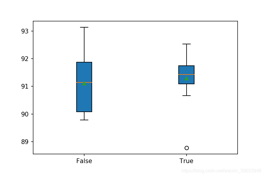
运行示例可能需要一段时间,具体取决于硬件,将为每个评估模型打印性能。运行结束时,总结每种测试配置的性能,并显示平均值和标准偏差。可以看到,在建模之前对数据集进行标准化确实会导致性能的小幅提升,从大约90.4%的准确性(接近上一节中看到的)提高到大约91.5%的准确性。
train_X.shape:(7352, 128, 9),train_y.shape:(7352, 1)

test_X.shape:(2947, 128, 9),test_y.shape:(2947, 1)

>p=False #1: 91.110
>p=False #2: 93.146
>p=False #3: 90.058
>p=False #4: 91.924
>p=False #5: 91.958
>p=False #6: 89.786
>p=False #7: 89.990
>p=False #8: 91.177
>p=False #9: 90.159
>p=False #10: 91.754
>p=True #1: 91.415
>p=True #2: 92.535
>p=True #3: 91.788
>p=True #4: 90.668
>p=True #5: 91.008
>p=True #6: 88.768
>p=True #7: 92.297
>p=True #8: 91.347
>p=True #9: 91.449
>p=True #10: 91.619
[[91.10960364341736, 93.14557313919067, 90.05768299102783, 91.923987865448, 91.95792078971863, 89.78622555732727, 89.98982310295105, 91.17746949195862, 90.15948176383972, 91.75432920455933], [91.41499996185303, 92.53478050231934, 91.78826212882996, 90.66847562789917, 91.00780487060547, 88.76823782920837, 92.29725003242493, 91.34713411331177, 91.44893288612366, 91.6185975074768]] [False, True]
Param=False: 91.106% (+/-1.047)
Param=True: 91.289% (+/-0.989)
还创建了结果的箱型图。这允许以非参数的方式比较两个结果样本,显示每个样本的中位数和中间50%。我们可以看到,具有标准化结果的分布与没有标准化结果的分布有很大不同。这可能是真实的效果。
2.3 filters 数量的影响
现在有了实验框架,可以探索该模型的其他超参数。 CNN的重要超参数是filter maps的数量,可以尝试各种不同的值,可以尝试以下数量的filter:
n_params = [8, 16, 32, 64, 128, 256]
完整代码:
from sklearn.preprocessing import StandardScaler
import pandas as pd
import numpy as np
import matplotlib.pyplot as plt
import os

from tensorflow.keras.models import Sequential
from tensorflow.keras.layers import Dense, Flatten, Dropout
from tensorflow.keras.layers import Conv1D, MaxPooling1D
from tensorflow.keras.utils import to_categorical

def load_file(filepath):
    dataframe = pd.read_csv(filepath, header=None, delim_whitespace=True)
    return dataframe.values

def load_dataset(data_rootdir, dirname, group):
    '''
    该函数实现将训练数据或测试数据文件列表堆叠为三维数组
    '''
    filename_list = []
    filepath_list = []
    X = []

    # os.walk() 方法是一个简单易用的文件、目录遍历器,可以高效的处理文件、目录。
    for rootdir, dirnames, filenames in os.walk(data_rootdir + dirname):
        for filename in filenames:
            filename_list.append(filename)
            filepath_list.append(os.path.join(rootdir, filename))
        #print(filename_list)
        #print(filepath_list)

    # 遍历根目录下的文件,并读取为DataFrame格式;
    for filepath in filepath_list:
        X.append(load_file(filepath))

    X = np.dstack(X) # dstack沿第三个维度叠加,两个二维数组叠加后,前两个维度尺寸不变,第三个维度增加;
    y = load_file(data_rootdir+'/y_'+group+'.txt')
    print('{}_X.shape:{},{}_y.shape:{}\n'.format(group,X.shape,group,y.shape))
    return X, y


def evaluate_model(trainX, trainy, testX, testy, n_filters):
    verbose, epochs, batch_size = 0, 10, 32

    n_timesteps, n_features, n_outputs = trainX.shape[1], trainX.shape[2], trainy.shape[1]

    model = Sequential()
    model.add(Conv1D(filters=n_filters, kernel_size=3, activation='relu',
                     input_shape=(n_timesteps,n_features)))
    model.add(Conv1D(filters=n_filters, kernel_size=3, activation='relu'))
    model.add(Dropout(0.5))
    model.add(MaxPooling1D(pool_size=2))
    model.add(Flatten())
    model.add(Dense(100, activation='relu'))
    model.add(Dense(n_outputs, activation='softmax'))
    model.compile(loss='categorical_crossentropy', optimizer='adam', metrics=['accuracy'])

    model.fit(trainX, trainy, epochs=epochs, batch_size=batch_size, verbose=verbose)

    _, accuracy = model.evaluate(testX, testy, batch_size=batch_size, verbose=0)
    return accuracy


def summarize_results(scores, params):
    print(scores, params)
    # 总结均值和标准差
    for i in range(len(scores)):
        m, s = np.mean(scores[i]), np.std(scores[i])
        print('Param=%s: %.3f%% (+/-%.3f)' % (params[i], m, s))
    # 绘制分数的箱型图
    plt.boxplot(scores, vert=True,  patch_artist=True, showmeans=True, labels=params)
    plt.savefig('exp_cnn_filters.png', dpi=150)
    plt.show()

def run_experiment(trainX, trainy, testX, testy, params, repeats=10):
    # one-hot编码
    # 这个之前的文章中提到了,因为原数据集标签从1开始,而one-hot编码从0开始,所以要先减去1
    trainy = to_categorical(trainy-1)
    testy = to_categorical(testy-1)

    all_scores = list()
    for p in params:

        scores = list()
        for r in range(repeats):
            score = evaluate_model(trainX, trainy, testX, testy, p)
            score = score * 100.0
            print('>p=%s #%d: %.3f' % (p, r+1, score))
            scores.append(score)
        all_scores.append(scores)

    summarize_results(all_scores, params)

train_dir = 'D:/GraduationCode/01 Datasets/UCI HAR Dataset/train/'
test_dir = 'D:/GraduationCode/01 Datasets/UCI HAR Dataset/test/'
dirname = '/Inertial Signals/'
trainX, trainy = load_dataset(train_dir, dirname, 'train')
testX, testy = load_dataset(test_dir, dirname, 'test')

n_params = [8, 16, 32, 64, 128, 256]
run_experiment(trainX, trainy, testX, testy, n_params, repeats=2)
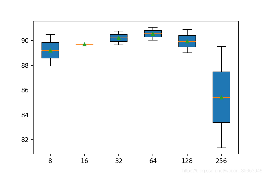
运行示例将对每个指定数量的滤波器(filters)重复实验。运行结束时,打印每个滤波器数量的结果摘要。可以看到随着滤波器图数量的增加,平均性能也有提高的趋势。方差保持相当恒定,也许对于网络来说128个特征图可能是一个很好的配置。
train_X.shape:(7352, 128, 9),train_y.shape:(7352, 1)

test_X.shape:(2947, 128, 9),test_y.shape:(2947, 1)

>p=8 #1: 90.465
>p=8 #2: 87.954
>p=16 #1: 89.718
>p=16 #2: 89.684
>p=32 #1: 89.650
>p=32 #2: 90.770
>p=64 #1: 91.076
>p=64 #2: 90.024
>p=128 #1: 90.872
>p=128 #2: 89.006
>p=256 #1: 81.337
>p=256 #2: 89.515
[[90.46487808227539, 87.95385360717773], [89.71835970878601, 89.68442678451538], [89.65049386024475, 90.77027440071106], [91.07567071914673, 90.0237500667572], [90.87207317352295, 89.00576829910278], [81.33695125579834, 89.51476216316223]] [8, 16, 32, 64, 128, 256]
Param=8: 89.209% (+/-1.256)
Param=16: 89.701% (+/-0.017)
Param=32: 90.210% (+/-0.560)
Param=64: 90.550% (+/-0.526)
Param=128: 89.939% (+/-0.933)
Param=256: 85.426% (+/-4.089)
还创建了结果的箱型图,从而可以比较每个滤波器数量的结果分布。从图中可以看出,随着特征图数量的增加,就中值分类精度(框上的橙色线)而言,趋势呈上升趋势。 filters=64时(我们实验中的默认值或基线)分类精度有所下降;在32,128和256时,准确性可能处于稳定状态。也许32是更稳定的配置。
2.4 kenel_size的影响
kernel的大小是要调整的1D CNN的另一个重要超参数。kernel大小控制着在每次读取输入序列时要考虑的时间步长,然后通过卷积过程将其映射到特征图上。较大的kernel大小意味着对数据的读取不太严格,但是可能导致输入的快照更加通用。除了默认的三个时间步长以外,我们可以使用相同的实验设置并测试一组不同的kernel大小。值的列表如下:
n_kernels = [2, 3, 5, 7, 11]
完整代码:
from sklearn.preprocessing import StandardScaler
import pandas as pd
import numpy as np
import matplotlib.pyplot as plt
import os

from tensorflow.keras.models import Sequential
from tensorflow.keras.layers import Dense, Flatten, Dropout
from tensorflow.keras.layers import Conv1D, MaxPooling1D
from tensorflow.keras.utils import to_categorical

def load_file(filepath):
    dataframe = pd.read_csv(filepath, header=None, delim_whitespace=True)
    return dataframe.values

def load_dataset(data_rootdir, dirname, group):
    '''
    该函数实现将训练数据或测试数据文件列表堆叠为三维数组
    '''
    filename_list = []
    filepath_list = []
    X = []

    # os.walk() 方法是一个简单易用的文件、目录遍历器,可以高效的处理文件、目录。
    for rootdir, dirnames, filenames in os.walk(data_rootdir + dirname):
        for filename in filenames:
            filename_list.append(filename)
            filepath_list.append(os.path.join(rootdir, filename))
        #print(filename_list)
        #print(filepath_list)

    # 遍历根目录下的文件,并读取为DataFrame格式;
    for filepath in filepath_list:
        X.append(load_file(filepath))

    X = np.dstack(X) # dstack沿第三个维度叠加,两个二维数组叠加后,前两个维度尺寸不变,第三个维度增加;
    y = load_file(data_rootdir+'/y_'+group+'.txt')
    print('{}_X.shape:{},{}_y.shape:{}\n'.format(group,X.shape,group,y.shape))
    return X, y


def evaluate_model(trainX, trainy, testX, testy, n_filters, n_kernel):
    verbose, epochs, batch_size = 0, 10, 32

    n_timesteps, n_features, n_outputs = trainX.shape[1], trainX.shape[2], trainy.shape[1]

    model = Sequential()
    model.add(Conv1D(filters=n_filters, kernel_size=n_kernel, activation='relu',
                     input_shape=(n_timesteps,n_features)))
    model.add(Conv1D(filters=n_filters, kernel_size=n_kernel, activation='relu'))
    model.add(Dropout(0.5))
    model.add(MaxPooling1D(pool_size=2))
    model.add(Flatten())
    model.add(Dense(100, activation='relu'))
    model.add(Dense(n_outputs, activation='softmax'))
    model.compile(loss='categorical_crossentropy', optimizer='adam', metrics=['accuracy'])

    model.fit(trainX, trainy, epochs=epochs, batch_size=batch_size, verbose=verbose)

    _, accuracy = model.evaluate(testX, testy, batch_size=batch_size, verbose=0)
    return accuracy


def summarize_results(scores, params):
    print(scores, params)
    # 总结均值和标准差
    for i in range(len(scores)):
        m, s = np.mean(scores[i]), np.std(scores[i])
        print('Param=%s: %.3f%% (+/-%.3f)' % (params[i], m, s))
    # 绘制分数的箱型图
    plt.boxplot(scores, vert=True,  patch_artist=True, showmeans=True, labels=params)
    plt.savefig('exp_cnn_kernels.png', dpi=150)
    plt.show()

def run_experiment(trainX, trainy, testX, testy, n_filters, params, repeats=10):
    # one-hot编码
    # 这个之前的文章中提到了,因为原数据集标签从1开始,而one-hot编码从0开始,所以要先减去1
    trainy = to_categorical(trainy-1)
    testy = to_categorical(testy-1)

    all_scores = list()
    for p in params:

        scores = list()
        for r in range(repeats):
            score = evaluate_model(trainX, trainy, testX, testy, n_filters, p)
            score = score * 100.0
            print('>p=%s #%d: %.3f' % (p, r+1, score))
            scores.append(score)
        all_scores.append(scores)

    summarize_results(all_scores, params)

train_dir = 'D:/GraduationCode/01 Datasets/UCI HAR Dataset/train/'
test_dir = 'D:/GraduationCode/01 Datasets/UCI HAR Dataset/test/'
dirname = '/Inertial Signals/'
trainX, trainy = load_dataset(train_dir, dirname, 'train')
testX, testy = load_dataset(test_dir, dirname, 'test')

#n_filters = [8, 16, 32, 64, 128, 256]
n_filters = 64
n_kernels = [2, 3, 5, 7, 11]
run_experiment(trainX, trainy, testX, testy, n_filters, n_kernels, repeats=2)
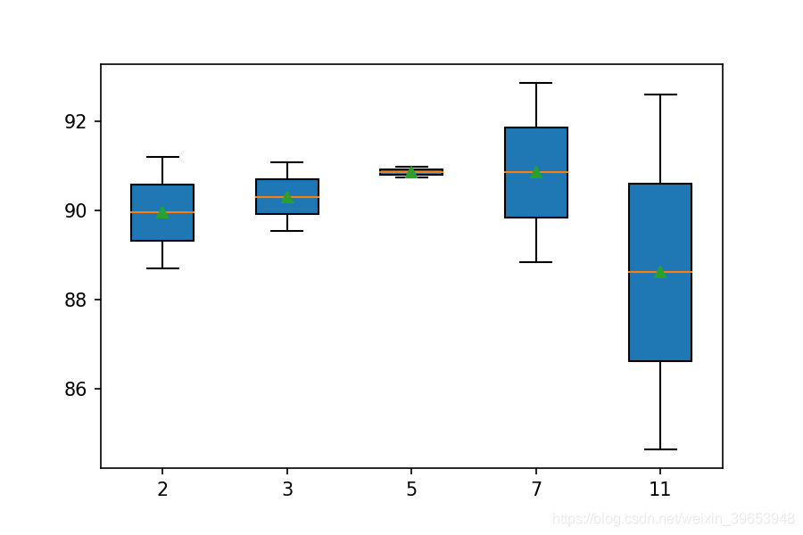
运行示例依次测试每个kernel大小,运行结束时汇总结果。我们可以看到,随着kernel大小的增加,模型性能总体上得到了提高。结果表明,kernel大小为5可能很好,平均技能约为91.8%,但7或11可能也同样有较小的标准偏差。
train_X.shape:(7352, 128, 9),train_y.shape:(7352, 1)

test_X.shape:(2947, 128, 9),test_y.shape:(2947, 1)

>p=2 #1: 88.700
>p=2 #2: 91.211
>p=3 #1: 91.076
>p=3 #2: 89.549
>p=5 #1: 90.736
>p=5 #2: 90.974
>p=7 #1: 88.836
>p=7 #2: 92.874
>p=11 #1: 92.603
>p=11 #2: 84.628
[[88.70037198066711, 91.21140241622925], [91.07567071914673, 89.54869508743286], [90.73634147644043, 90.97387194633484], [88.83610367774963, 92.87410974502563], [92.6026463508606, 84.62843298912048]] [2, 3, 5, 7, 11]
Param=2: 89.956% (+/-1.256)
Param=3: 90.312% (+/-0.763)
Param=5: 90.855% (+/-0.119)
Param=7: 90.855% (+/-2.019)
Param=11: 88.616% (+/-3.987)
还创建了箱型图。结果表明,较大的kernel大小确实有更高的准确性,并且kernel大小为7时,可以在良好性能和低方差之间提供良好的平衡。
以上只是比较简单的调参,探索上述参数的组合重新测试,看看性能是否可以进一步提升。也可以将重复次数从10增加到30甚至更多,以查看其结果是否更稳定。
3. Multi-head CNN 模型
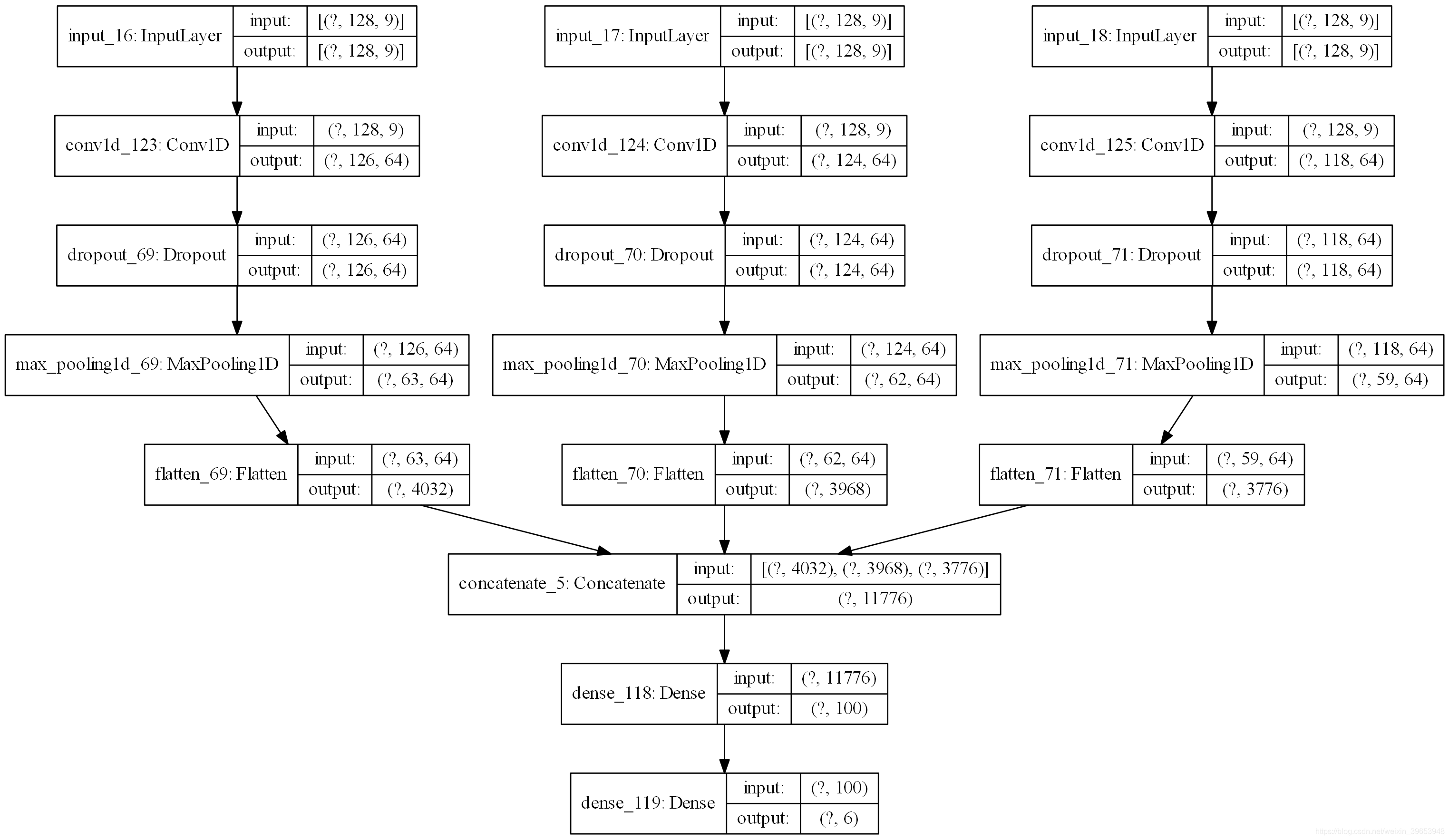
一维CNN的另一种流行方法是使用multi-head模型,其中模型的每个head可以使用不同大小的kernel读取输入时间步长。例如,三个head的模型可以具有3、5、11的三个不同的kernel大小,从而允许模型以三种不同的分辨率读取和解释序列数据。然后,在做出预测之前,将来自所有三个头的解释连接到模型中,并由全连接层进行解释。可以使用Keras Function API实现 Multi-head 1D CNN。该模型的其他方面可能会因情况而异,例如滤波器的数量,甚至数据本身的准备。下面列出了Multi-head 1D CNN的完整代码。创建模型时,将创建网络结构图。
注意:调用 plot model() 需要安装 pygraphviz 和 pydot 。
完整代码:
import pandas as pd
import numpy as np
import matplotlib.pyplot as plt
import os

from tensorflow.keras.models import Model
from tensorflow.keras.layers import Input, Dense, Flatten, Dropout
from tensorflow.keras.layers import Conv1D, MaxPooling1D
from tensorflow.keras.layers import concatenate
from tensorflow.keras.utils import to_categorical, plot_model

def load_file(filepath):
    dataframe = pd.read_csv(filepath, header=None, delim_whitespace=True)
    return dataframe.values

def load_dataset(data_rootdir, dirname, group):
    '''
    该函数实现将训练数据或测试数据文件列表堆叠为三维数组
    '''
    filename_list = []
    filepath_list = []
    X = []

    # os.walk() 方法是一个简单易用的文件、目录遍历器,可以高效的处理文件、目录。
    for rootdir, dirnames, filenames in os.walk(data_rootdir + dirname):
        for filename in filenames:
            filename_list.append(filename)
            filepath_list.append(os.path.join(rootdir, filename))
        #print(filename_list)
        #print(filepath_list)

    # 遍历根目录下的文件,并读取为DataFrame格式;
    for filepath in filepath_list:
        X.append(load_file(filepath))

    X = np.dstack(X) # dstack沿第三个维度叠加,两个二维数组叠加后,前两个维度尺寸不变,第三个维度增加;
    y = load_file(data_rootdir+'/y_'+group+'.txt')
    print('{}_X.shape:{},{}_y.shape:{}\n'.format(group,X.shape,group,y.shape))
    return X, y

def evaluate_model(trainX, trainy, testX, testy):
    verbose, epochs, batch_size = 0, 10, 32
    n_timesteps, n_features, n_outputs = trainX.shape[1], trainX.shape[2], trainy.shape[1]

    # head 1
    inputs1 = Input(shape=(n_timesteps,n_features))
    conv1 = Conv1D(filters=64, kernel_size=3, activation='relu')(inputs1)
    drop1 = Dropout(0.5)(conv1)
    pool1 = MaxPooling1D(pool_size=2)(drop1)
    flat1 = Flatten()(pool1)

    # head 2
    inputs2 = Input(shape=(n_timesteps,n_features))
    conv2 = Conv1D(filters=64, kernel_size=5, activation='relu')(inputs2)
    drop2 = Dropout(0.5)(conv2)
    pool2 = MaxPooling1D(pool_size=2)(drop2)
    flat2 = Flatten()(pool2)

    # head 3
    inputs3 = Input(shape=(n_timesteps,n_features))
    conv3 = Conv1D(filters=64, kernel_size=11, activation='relu')(inputs3)
    drop3 = Dropout(0.5)(conv3)
    pool3 = MaxPooling1D(pool_size=2)(drop3)
    flat3 = Flatten()(pool3)

    # 合并
    merged = concatenate([flat1, flat2, flat3])
    # 解释
    dense1 = Dense(100, activation='relu')(merged)
    outputs = Dense(n_outputs, activation='softmax')(dense1)
    model = Model(inputs=[inputs1, inputs2, inputs3], outputs=outputs)

    plot_model(model, show_shapes=True, to_file='multichannel.png', dpi=200)
    model.compile(loss='categorical_crossentropy', optimizer='adam', metrics=['accuracy'])

    model.fit([trainX,trainX,trainX], trainy, epochs=epochs, batch_size=batch_size, verbose=verbose)

    _, accuracy = model.evaluate([testX,testX,testX], testy, batch_size=batch_size, verbose=0)
    return accuracy

def run_experiment(trainX, trainy, testX, testy, repeats=10):
    # one-hot编码
    # 这个之前的文章中提到了,因为原数据集标签从1开始,而one-hot编码从0开始,所以要先减去1
    trainy = to_categorical(trainy-1)
    testy = to_categorical(testy-1)

    scores = []
    for r in range(repeats):
        score = evaluate_model(trainX, trainy, testX, testy)
        score = score * 100.0
        print('>#%d: %.3f' % (r+1, score))
        scores.append(score)
        print(scores)

    mean_scores, std_scores = np.mean(scores), np.std(scores)
    print('Accuracy: %.3f%% (+/-%.3f)' % (mean_scores, std_scores))

train_dir = 'D:/GraduationCode/01 Datasets/UCI HAR Dataset/train/'
test_dir = 'D:/GraduationCode/01 Datasets/UCI HAR Dataset/test/'
dirname = '/Inertial Signals/'
trainX, trainy = load_dataset(train_dir, dirname, 'train')
testX, testy = load_dataset(test_dir, dirname, 'test')
run_experiment(trainX, trainy, testX, testy, repeats=5)
运行示例将打印实验的每个重复步骤的模型性能,然后将估计分数汇总为均值和标准差。可以看到,模型的平均性能约为90.9%的分类精度,标准偏差约为2.7(可以多增加repeat数量,我只试验了两次)。该示例可以用作探索各种其他模型的基础,可以改变子模型的超参数,不同的数据准备方案。
train_X.shape:(7352, 128, 9),train_y.shape:(7352, 1)

test_X.shape:(2947, 128, 9),test_y.shape:(2947, 1)

>#1: 91.822
[91.82218909263611]
>#2: 92.501
[91.82218909263611, 92.5008475780487]
>#3: 91.686
[91.82218909263611, 92.5008475780487, 91.68646335601807]
>#4: 85.579
[91.82218909263611, 92.5008475780487, 91.68646335601807, 85.57855486869812]
>#5: 93.044
[91.82218909263611, 92.5008475780487, 91.68646335601807, 85.57855486869812, 93.04377436637878]
Accuracy: 90.926% (+/-2.718)
网络架构:

4. 扩展
以下是一些扩展教程的想法。
- 变量数(特征数)。进行实验查看CNN中是否需要全部九个变量,或者它是否可以对子集(例如总加速度)做得更好或更好。
- 数据准备。探索其他数据准备方案,例如数据标准化以及标准化后的标准化。探索其他网络架构,例如更深的CNN架构和更深的全连接层,以解释CNN输入功能。
- 诊断。使用简单的学习曲线诊断程序来解释模型在各个时期的学习方式,以及更多的正则化,不同的学习率,不同的批次大小或时期数是否可能导致性能更好或更稳定的模型。
下篇内容介绍LSTM模型及相关变体实现人类行为识别任务。


 被折叠的 条评论
为什么被折叠?
被折叠的 条评论
为什么被折叠?
 到【灌水乐园】发言


