pandas describe函数_Python连载|Pandas统计基本功能（一）

上一期给大家介绍了pandas的两大主要结构，相信大家对Series及DataFrame的创建和使用都比较熟悉了，那么接下来的两期将介绍pandas中的统计基本功能。学习完这部分内容后，相信你已能够轻松应对大部分的数据处理操作~

1 Pandas描述性统计

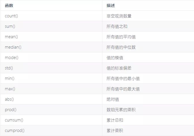
在Pandas中，可以使用描述性统计函数获取数据的描述统计信息，也可以使用 describe()函数查看DataFrame中所有数据每列的描述统计信息。Pandas中描述性统计信息的函数如下：

具体请看下面的例子

# 生成样例数据

d = {'A':pd.Series(['T','J','R','V','S','M','Z',

'L','D','G','B','A']),

'B':pd.Series([25,26,25,23,30,29,23,34,40,30,51,46]),

'C':pd.Series([4.23,3.24,3.98,2.56,3.20,4.6,3.8,3.78,2.98,4.80,4.10,3.65])}

df = pd.DataFrame(d)

print(df.sum()) # 对每一列进行求和

print(df.sum(axis=1)) # 对每一行进行求和

print(df.mean()) # 返回平均值

print(df.std()) # 返回数字列的标准偏差

print(df.describe()) # 默认情况下只统计数值列

print(df.describe(include='all')) # 将所有列汇总在一起

输出结果：

#df.sum()

A TJRVSMZLDGBA

B 382

C 44.92

dtype: object

#df.sum(axis=1)

0 29.23

1 29.24

2 28.98

3 25.56

4 33.20

5 33.60

6 26.80

7 37.78

8 42.98

9 34.80

10 55.10

11 49.65

dtype: float64

#df.mean()

Age 31.833333

Rating 3.743333

dtype: float64

#df.std()

Age 9.232682

Rating 0.661628

dtype: float64

#df.describe()

B C

count 12.000000 12.000000

mean 31.833333 3.743333

std 9.232682 0.661628

min 23.000000 2.560000

25% 25.000000 3.230000

50% 29.500000 3.790000

75% 35.500000 4.132500

max 51.000000 4.800000

#df.describe(include='all'))

A B C

count 12 12.000000 12.000000

unique 12 NaN NaN

top S NaN NaN

freq 1 NaN NaN

mean NaN 31.833333 3.743333

std NaN 9.232682 0.661628

min NaN 23.000000 2.560000

25% NaN 25.000000 3.230000

50% NaN 29.500000 3.790000

75% NaN 35.500000 4.132500

max NaN 51.000000 4.800000

2 Pandas函数应用

2.1 Pandas统计函数

2.1.1 pct_change()函数

Series，DatFrames都有pct_change()函数。此函数表示当前元素与前面元素的相差百分比。

s = pd.Series([1,3,2,1])

s.pct_change()

输出结果：

0 NaN

1 2.000000

2 -0.333333

3 -0.500000

dtype: float64

2.1.2 协方差

可用cov来计算Series对象之间的协方差。

# 计算过程中NA将被自动排除

s1 = pd.Series(np.random.randn(5))

s2 = pd.Series(np.random.randn(5))

s1.cov(s2) #0.10128793423437038

当应用于DataFrame时，协方差方法计算所有列之间的协方差值

f = pd.DataFrame(np.random.randn(10,3),columns=['a','b','c'])

f.cov()

输出结果：

a b c

a 0.842634 -0.297079 0.522180

b -0.297079 0.840638 0.150882

c 0.522180 0.150882 1.081326

2.1.3 相关性

相关性显示了任何两个数值(Series)之间的线性关系,其计算方法有pearson,spearman 和 kendall相关性。其中默认为Pearson相关系数。如果DataFrame中存在任何非数字列，则会自动排除

f.corr() # 计算Pearson相关系数

输出结果：

a b c

a 1.000000 -0.352978 0.547045

b -0.352978 1.000000 0.158254

c 0.547045 0.158254 1.000000

2.1.4 数据排名

数据排名为元素数组中的每个元素生成排名。rank()默认为true的升序排列; 当False时，数据按反序排列。rank支持不同的排序方法，具体如下面例子所示

s = pd.Series(np.random.np.random.randn(5),index=list('abcde'))

s['d'] = s['b'] # 构造一个相同的情况

print(s.rank())

print(s.rank(method='min')) # 使用min方法后，比如有两个排名并列第三，则两个的排名都为3

print(s.rank(method='max')) # 使用max方法后，比如有两个排名并列第三，则两个数的排名都为4

print(s.rank(method='first')) # 数值大小相同情况下，根据在数组中的位置来定排名前后

输出结果：

#s.rank()

a 5.0

b 3.5

c 2.0

d 3.5

e 1.0

dtype: float64

#s.rank(method='min')

a 5.0

b 3.0

c 2.0

d 3.0

e 1.0

dtype: float64

#s.rank(method='max')

a 5.0

b 4.0

c 2.0

d 4.0

e 1.0

dtype: float64

#s.rank(method='first')

a 5.0

b 3.0

c 2.0

d 4.0

e 1.0

dtype: float64

2.2 Pandas窗口函数

Pandas提供了滚动，展开等窗口函数，方便对时间序列数据进行处理。

2.2.1 .rolling()函数

该函数可应用于一系列数据，并按指定周期计算

# 构建样例数据

df = pd.DataFrame(np.random.randn(10,4),

index = pd.date_range('1/1/2019',periods=10),

columns = ['A','B','C','D'])

print(df)

print(df.rolling(window=3).mean()) # 由于窗口大小为3，前两个元素为空值，第三个元素的值为n，n-1,n-2元素的平均值

输出结果：

#df

A B C D

2019-01-01 -1.327987 0.663651 1.631045 -0.042281

2019-01-02 -0.005253 0.420348 0.442055 -0.218387

2019-01-03 0.356261 0.755611 -0.105040 -1.126363

2019-01-04 0.853231 -0.272414 1.696901 -0.336484

2019-01-05 -0.432228 -2.321604 -0.300705 0.965461

2019-01-06 0.032065 0.464344 1.346653 -0.127116

2019-01-07 -0.988206 -1.518681 0.443509 1.601487

2019-01-08 -0.396659 2.169251 -0.342024 -1.092281

2019-01-09 0.380469 -1.009371 0.117781 -0.157493

2019-01-10 -1.792407 -1.456297 -1.377632 1.093072

#df.rolling(window=3).mean()

A B C D

2019-01-01 NaN NaN NaN NaN

2019-01-02 NaN NaN NaN NaN

2019-01-03 -0.325660 0.613203 0.656020 -0.462344

2019-01-04 0.401413 0.301181 0.677972 -0.560411

2019-01-05 0.259088 -0.612802 0.430385 -0.165796

2019-01-06 0.151023 -0.709891 0.914283 0.167287

2019-01-07 -0.462790 -1.125313 0.496486 0.813277

2019-01-08 -0.450933 0.371638 0.482713 0.127363

2019-01-09 -0.334799 -0.119600 0.073089 0.117237

2019-01-10 -0.602865 -0.098806 -0.533958 -0.052234

2.2.2 .expanding()函数

expanding和rolling类似，只是expanding不是固定窗口长度，它的长度是不断扩大的。

df.expanding(min_periods=3).mean() # 第n个结果值为 第1,2，..，n-1的值求和再求平均

输出结果：

A B C D

2019-01-01 NaN NaN NaN NaN

2019-01-02 NaN NaN NaN NaN

2019-01-03 -0.325660 0.613203 0.656020 -0.462344

2019-01-04 -0.030937 0.391799 0.916240 -0.430879

2019-01-05 -0.111195 -0.150882 0.672851 -0.151611

2019-01-06 -0.087319 -0.048344 0.785151 -0.147529

2019-01-07 -0.216017 -0.258392 0.736345 0.102331

2019-01-08 -0.238597 0.045063 0.601549 -0.046996

2019-01-09 -0.169812 -0.072096 0.547797 -0.059273

2019-01-10 -0.332071 -0.210516 0.355254 0.055961

2.3 Pandas其他函数应用

Pandas函数应用主要有以下几方面的运用：

• 行或列函数应用：apply()

• 元素函数应用：applymap()

2.3.1 apply

可以使用apply()方法沿DataFrame的轴应用任意函数。默认情况下，操作按列执行，将每列列为数组。

df = pd.DataFrame(np.random.randn(5,3),columns=['col1','col2','col3'])

print(df.apply(np.mean))

print(df.apply(np.mean,axis=1))

print(df.apply(lambda x:x.max() - x.min()))

输出结果：

# df.apply(np.mean)

col1 0.324740

col2 1.023603

col3 -0.097148

dtype: float64

# df.apply(np.mean,axis=1)

0 0.883146

1 0.500423

2 -0.016306

3 -0.588286

4 1.306348

dtype: float64

# df.apply(lambda x:x.max() - x.min())

col1 1.750537

col2 4.022997

col3 2.924760

dtype: float64

2.3.2 applymap

在DataFrame上的方法applymap()类似于在Series上的map()接受任何Python函数，并且返回单个值。applymap对DataFrame中的每个值进行操作。

print(df['col1'].map(lambda x:x*100))# map针对于Series

print(df.applymap(lambda x:x*100))# applymap针对DataFrame

输出结果：

#df['col1'].map(lambda x:x*100)

0 -32.095232

1 136.731397

2 48.233763

3 -38.322272

4 47.822448

Name: col1, dtype: float64

#df.applymap(lambda x:x*100)

col1 col2 col3

0 -32.095232 340.825931 -43.786954

1 136.731397 -3.286422 16.681865

2 48.233763 65.502181 -118.627596

3 -38.322272 -61.473778 -76.689607

4 47.822448 170.233595 173.848357

3 数据运算

3.1 Series之间的运算

m = pd.Series([1,2,3,4],index=['a','b','c','d'])

n = pd.Series([1,-1,3,-7,-2],index=['a','e','c','f','g'])

print(m,n,m+n,m-n,m*n,m/n)

输出结果：

# m

a 1

b 2

c 3

d 4

dtype: int64

# n

a 1

e -1

c 3

f -7

g -2

dtype: int64

# m+n

a 2.0

b NaN

c 6.0

d NaN

e NaN

f NaN

g NaN

dtype: float64

# m-n

a 0.0

b NaN

c 0.0

d NaN

e NaN

f NaN

g NaN

dtype: float64

# m*n

a 1.0

b NaN

c 9.0

d NaN

e NaN

f NaN

g NaN

dtype: float64

# m/n

a 1.0

b NaN

c 1.0

d NaN

e NaN

f NaN

g NaN

dtype: float64

sereis相加会自动进行数据对齐操作，在不重叠的索引处会使用NA(NaN)值进行填充，series进行算术运算的时候，不需要保证series的大小一致。其余操作类似。

3.2 DataFrame之间的运算

dataFrame相加时，对齐操作需要行和列的索引都重叠的时候才会相加，否则会使用NA值进行填充。其他操作类似

d1 = np.arange(1,10).reshape(3,3)

data1 = pd.DataFrame(d1,index=["a","b","c"],columns=["one","two","three"])

d2 = np.arange(1,10).reshape(3,3)

data2 = pd.DataFrame(d2,index=["a","b","e"],columns=["one","two","four"])

print(data1 + data2,data1 - data2,data1 * data2,data1 / data2)

输出结果：

# data1 + data2

four one three two

a NaN 2.0 NaN 4.0

b NaN 8.0 NaN 10.0

c NaN NaN NaN NaN

e NaN NaN NaN NaN

# data1 - data2

four one three two

a NaN 0.0 NaN 0.0

b NaN 0.0 NaN 0.0

c NaN NaN NaN NaN

e NaN NaN NaN NaN

# data1 * data2

four one three two

a NaN 1.0 NaN 4.0

b NaN 16.0 NaN 25.0

c NaN NaN NaN NaN

e NaN NaN NaN NaN

# data1 / data2

four one three two

a NaN 1.0 NaN 1.0

b NaN 1.0 NaN 1.0

c NaN NaN NaN NaN

e NaN NaN NaN NaN

3.3 DataFrame与Series的混合运算

除了Series之间、DataFrame之间的运算外，pandas还支持DataFrame与Series的混合运算

# DataFrame的行进行广播

a = np.arange(9).reshape(3,3)

d = pd.DataFrame(a,index=['a','b','c'],columns=['one','two','three'])

s = d.ix[0]# 取d的第一行为Series

print(d + s) # dataframe每一行都与第一行的数值相加

a = d['one']

print(d.add(a,axis=0)) # dataframe每一列都与第一列的数值相加

输出结果：

#d + s

one two three

a 0 2 4

b 3 5 7

c 6 8 10

#d.add(a,axis=0)

one two three

a 0 1 2

b 6 7 8

c 12 13 14

4 pandas分组与聚合

4.1 分组

任何分组(groupby)操作都涉及原始对象的以下操作之一：

• 分割对象

• 应用一个函数

• 结合的结果

可以通过下面的方法来构建分组对象

# 构建样例数据

group_data = {'A': ['abc', 'abc', 'def', 'def', 'kk',

'xyz', 'kk', 'kk', 'abc', 'xyz', 'xyz', 'abc'],

'B': [1, 2, 2, 3, 3,4 ,1 ,1,2 , 4,1,2],

'Year': [2014,2015,2014,2015,2014,2015,2016,2017,2016,2014,2015,2017],

'P':[996,789,863,673,881,812,756,788,694,701,804,550]}

df = pd.DataFrame(group_data)

df.groupby('A') # 按A来分组

4.1.1 查看分组

调用.groups方法可以查看分组信息

print(df.groupby('A').groups) # 按单列分组

print(df.groupby(['A','Year']).groups) # 按多列分组

输出结果：

#df.groupby('A').groups

{'abc': Int64Index([0, 1, 8, 11], dtype='int64'),

'def': Int64Index([2, 3], dtype='int64'),

'kk': Int64Index([4, 6, 7], dtype='int64'),

'xyz': Int64Index([5, 9, 10], dtype='int64')}

#df.groupby(['A','Year']).groups

{('abc', 2014): Int64Index([0], dtype='int64'),

('abc', 2015): Int64Index([1], dtype='int64'),

('abc', 2016): Int64Index([8], dtype='int64'),

('abc', 2017): Int64Index([11], dtype='int64'),

('def', 2014): Int64Index([2], dtype='int64'),

('def', 2015): Int64Index([3], dtype='int64'),

('kk', 2014): Int64Index([4], dtype='int64'),

('kk', 2016): Int64Index([6], dtype='int64'),

('kk', 2017): Int64Index([7], dtype='int64'),

('xyz', 2014): Int64Index([9], dtype='int64'),

('xyz', 2015): Int64Index([5, 10], dtype='int64')}

4.1.2 迭代遍历分组

对于groupby对象，可以遍历类似itertools.obj的对象：

grouped = df.groupby('Year')

for name,group in grouped:

print(name)

print(group)

输出结果：

2014

A B Year P

0 abc 1 2014 996

2 def 2 2014 863

4 kk 3 2014 881

9 xyz 4 2014 701

2015

A B Year P

1 abc 2 2015 789

3 def 3 2015 673

5 xyz 4 2015 812

10 xyz 1 2015 804

2016

A B Year P

6 kk 1 2016 756

8 abc 2 2016 694

2017

A B Year P

7 kk 1 2017 788

11 abc 2 2017 550

使用get_group()方法，可以选择一个组。

grouped = df.groupby('Year')

print(grouped.get_group(2014)) # 使用get_group()方法，可以选择一个组。

print(df.groupby('Year').mean()) # 按Year列分组，获取其他列均值

print(df.groupby(['Year','Team']).mean())# 按多列分组，并获取其他列的均值

输出结果：

# grouped.get_group(2014)

A B Year P

0 abc 1 2014 996

2 def 2 2014 863

4 kk 3 2014 881

9 xyz 4 2014 701

# df.groupby('Year').mean()

B P

Year

2014 2.5 860.25

2015 2.5 769.50

2016 1.5 725.00

2017 1.5 669.00

# df.groupby(['Year','A']).mean()

B P

Year A

2014 abc 1.0 996.0

def 2.0 863.0

kk 3.0 881.0

xyz 4.0 701.0

2015 abc 2.0 789.0

def 3.0 673.0

xyz 2.5 808.0

2016 abc 2.0 694.0

kk 1.0 756.0

2017 abc 2.0 550.0

kk 1.0 788.0

也可以分组后，选择列进行运算：

g = df.groupby('Year') # 先按Year列分组

g['P'].mean() # 再对分组后的P列进行求均值

输出结果：

Year

2014 860.25

2015 769.50

2016 725.00

2017 669.00

Name: P, dtype: float64

4.2 聚合

聚合函数为每个组返回单个聚合值。当创建了分组(group by)对象，就可以对分组数据执行多个聚合操作。比较常用的是使用agg

grouped = df.groupby('Year')

grouped['P'].agg(np.sum)

输出结果：

Year

2014 3441

2015 3078

2016 1450

2017 1338

Name: P, dtype: int64

4.2.1 转换

transform能返回完整数据的某一变换。输出的形状和输入一致。

g = df.groupby('A')

score = lambda x: (x - x.mean()) / x.std()*10

g.transform(score)

输出结果：

B Year P

0 -15.000000 -11.618950 12.763989

1 5.000000 -3.872983 1.697410

2 -7.071068 -7.071068 7.071068

3 7.071068 7.071068 -7.071068

4 11.547005 -10.910895 11.190971

5 5.773503 5.773503 6.407580

6 -5.773503 2.182179 -8.059553

7 -5.773503 8.728716 -3.131418

8 5.000000 3.872983 -3.381455

9 5.773503 -11.547005 -11.522876

10 -11.547005 5.773503 5.115295

11 5.000000 11.618950 -11.079944

4.2.2 过滤

filter()函数用于过滤数据。根据定义的标准过滤数据,并返回数据的子集

f = df.groupby('A').filter(lambda x: len(x)>2) #筛选出特定条件的组

df.groupby('Team').filter(lambda x: np.max(x['B'])<=3) # 筛选出组中最大排名不超过3的组

输出结果：

A B Year P

0 abc 1 2014 996

1 abc 2 2015 789

2 def 2 2014 863

3 def 3 2015 673

4 kk 3 2014 881

6 kk 1 2016 756

7 kk 1 2017 788

8 abc 2 2016 694

11 abc 2 2017 550

---

至此，本次分享已结束 如果你喜欢的话，可以转发或者点个“在看”支持一下~ 点击原文链接，可以下载《Python工具代码速查手册》，可以点个star支持一下哦~ 简介：浩彬老撕 好玩的数据炼丹师， 曾经的IBM数据挖掘攻城狮， 还没开始就过气数据科学界的段子手， 致力于数据科学知识分享，不定期送书活动