matlab pca函数_pca+svm手写数字识别

本文采用pca算法提取图像特征，然后再用svm进行分类。

主要分为两步：

1、pca特征提取

pca主成份分析，主要用来进行人脸识别，具体原理介绍可以参考这篇博客http://blog.codinglabs.org/articles/pca-tutorial.html ，提取pca特征主要有以下几个步骤：

（1）将图像归一化到固定大小n*n，然后展开为1*n^2的一维向量，假设有m个样本，则最终形成一个m*n^2的数组，每一行代表一个样本，本文所用的图像大小为28*28，样本类别为10，每个类别训练图为500张，则每一张图展开后就是一个1*756的一维向量，最终形成一个5000*756的数组dm；

（2）求每一个列向量的均值avg，其大小为1*n^2；

（3）差值a=dm-avg；

（4）协方差b=a*a’；

（5）求协方差矩阵b的特征值和特征向量，取前k个最大特征值及对应的特征向量T；

（6）令c=a’*T，c的大小为n^2*k，向量c则为原始图像到投影空间的投影向量；

（7）投影向量p=dm*c为样本的特征向量，其大小为m*k，即将一个n*n大小的图像映射为一个1*k的向量，每一行代表一个样本；

（8）将求得的投影向量p送到svm分类器中进行训练。

识别的时候，只需要将待识别的图像d（1*n^2）先减去均值avg，再与投影向量c相乘，即将原始图像d投影到其主成份分量所在的投影空间中，然后用训练好的svm模型进行识别。 matlab自带pca的函数，可以直接调用，当然也可以自己实现pca，过程也比较简单。

2、svm分类

libsvm中实现多分类采用的是one-versus-one法，参照http://blog.csdn.net/liulina603/article/details/8498759 。

整个流程的代码如下：

clear;clc;
% 训练样本数量10*500
train_count=10;
train_count_per_num=500;
% 能量
energy=90;
train_path_mask='F:MATLABR2014aworklibsvm-3.11datashouxiepca_svmtrain%01d%01d.bmp';
training_samples=[];
train_label=[];%训练标签

% img_size=10;% 归一化图像大小
% 训练，自带的pca函数
tic
for i=0:train_count-1
    for j=1:train_count_per_num
        img=imread(sprintf(train_path_mask,i,j));
%         img=imresize(img,[img_size img_size]); % 归一化
        if ndims(img)==3
            img=rgb2gray(img);
        end
        img=im2bw(img,5/255);
        training_samples=[training_samples;img(:)'];
    end    
    train_label(i*train_count_per_num+1:(i+1)*train_count_per_num)=ones(1,train_count_per_num)*i;
end
training_samples=double(training_samples);%一定要转double
train_label=train_label';  %训练的标签
% mu=mean(training_samples); %训练集中的平均值
[train_coeff,train_scores,~,~,train_explained,mu]=pca(training_samples); %pca
train_idx=find(cumsum(train_explained)>energy,1); %idx为前k个特征向量,explained特征值
train_coeff=train_coeff(:,1:train_idx); %投影向量
train_img_arr=train_scores(:,1:train_idx); %特征向量，训练的样本集

%svm训练
model = svmtrain(train_label, train_img_arr, '-s 0 -c 1.5 -t 0 -g 3'); 
save('shouxie_model','model'); %保存svm模型
xlswrite('train_coeff.xlsx',train_coeff); %保存特征向量
xlswrite('mu.xlsx',mu); %保存样本平均值，单样本进行测试的时候会用到

%使用训练集数据进行测试
[train_predict_label, train_accuracy, train_dec_values] =svmpredict(train_label, train_img_arr, model); % test the trainingdata

%测试
test_path_mask='F:MATLABR2014aworklibsvm-3.11datashouxiepca_svmtest%01d%01d.bmp';
test_count=10;
test_count_per_num=100;
test_samples=[];
test_label=[];
for i=0:test_count-1
    for j=1:test_count_per_num
        img=imread(sprintf(test_path_mask,i,j));
%         img=imresize(img,[img_size img_size]); % 归一化
        if ndims(img)==3
            img=rgb2gray(img);
        end
        img=im2bw(img,5/255);
        test_samples=[test_samples;img(:)'];
    end    
    test_label(i*test_count_per_num+1:(i+1)*test_count_per_num)=ones(1,test_count_per_num)*i;
end
test_samples=double(test_samples);
test_label=test_label';
% test_img_arr=test_samples(:)-mu;
test_mu=repmat(mu,1000,1);
test_img_arr=test_samples-test_mu;
test_img_arr=test_img_arr*train_coeff; %测试集数据投影到投影向量上

%svm测试
[test_predict_label, test_accuracy, test_dec_values] =svmpredict(test_label, test_img_arr, model); 
toc

% test_img1=imread('F:MATLABR2014aworklibsvm-3.11datashouxiepca_svmtest010.bmp');
% % test_img1=imresize(test_img1,[img_size img_size]);
% test_img1=rgb2gray(test_img1);
% test_img1=im2bw(test_img1,5/255);
% test_img1=double(test_img1);
% test_img_arr1=test_img1(:)'-mu;
% test_img_arr=test_img_arr1*train_coeff;
% [predict_label, accuracy, dec_values] =svmpredict(1, test_img_arr, model);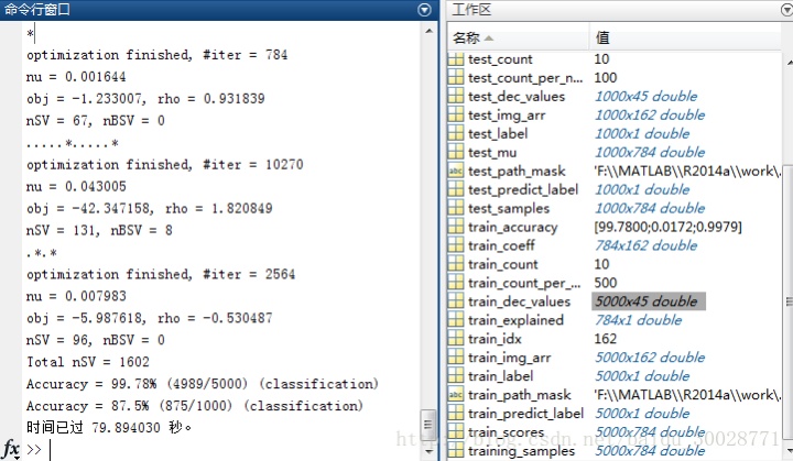 

用训练样本进行测试的时候，Accuracy = 99.78% (4989/5000) ，用新的测试集时， Accuracy = 87.5% (875/1000)，比直接使用原始图进行训练高多了，当然，其精度还可以进一步提升。改变-s -c -t -g 等参数进行训练时，可能会出现过拟合、欠拟合等情况，需要多次尝试确定其合适的参数值大小。参数调优可以参照这篇博客http://blog.csdn.net/chunxiao2008/article/details/50448154 。

3、参数讲解

在使用libsvm工具箱的时候，主要用到了svmtrain、svmpredict两个函数，现在介绍下其中的几个重要的参数。

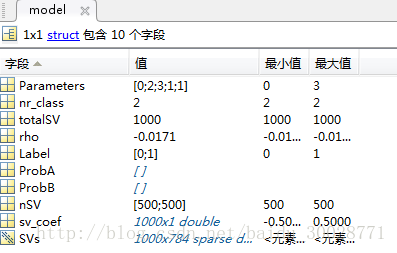
使用svmtrain后会得到一个model，参数如下：

model.Parameters参数意义从上到下依次为，在svmtrain函数可以通过字符串进行设置：

 -s svm类型：SVM设置类型(默认0) 
 -t 核函数类型：核函数设置类型(默认2) 
 -d degree：核函数中的degree设置(针对多项式核函数)(默认3) 
 -g r(gama)：核函数中的gamma函数设置(针对多项式/rbf/sigmoid核函数) (默认类别数目的倒数) 
 -r coef0：核函数中的coef0设置(针对多项式/sigmoid核函数)((默认0)。
具体解释可以在readme文档中查看， 
 options: 
-s svm_type : set type of SVM (default 0) 
 0 – C-SVC 
 1 – nu-SVC 
 2 – one-class SVM 
 3 – epsilon-SVR 
 4 – nu-SVR 
-t kernel_type : set type of kernel function (default 2) 
 0 – linear: u’*v 
 1 – polynomial: (gamma*u’*v + coef0)^degree 
 2 – radial basis function: exp(-gamma*|u-v|^2) 
 3 – sigmoid: tanh(gamma*u’*v + coef0) 
 4 – precomputed kernel (kernel values in training_set_file)
-d degree : set degree in kernel function (default 3)–核函数中的degree设置(针对多项式核函数)(默认3) 
 -g gamma : set gamma in kernel function (default 1/num_features)–核函数中的gamma函数设置(针对多项式/rbf/sigmoid核函数)(默认1/ k) 
 -r coef0 : set coef0 in kernel function (default 0)–核函数中的coef0设置(针对多项式/sigmoid核函数)((默认0) 
 -c cost : set the parameter C of C-SVC, epsilon-SVR, and nu-SVR (default 1)–设置C-SVC，e -SVR和v-SVR的参数(损失函数)(默认1) 
 -n nu : set the parameter nu of nu-SVC, one-class SVM, and nu-SVR (default 0.5)–设置v-SVC，一类SVM和v- SVR的参数(默认0.5) 
 -p epsilon : set the epsilon in loss function of epsilon-SVR (default 0.1)–设置e -SVR 中损失函数p的值(默认0.1) 
 -m cachesize : set cache memory size in MB (default 100)–设置cache内存大小，以MB为单位(默认100) 
 -e epsilon : set tolerance of termination criterion (default 0.001)–设置允许的终止判据(默认0.001)
-h shrinking : whether to use the shrinking heuristics, 0 or 1 (default 1)–是否使用启发式，0或1(默认1) 
 -b probability_estimates : whether to train a SVC or SVR model for probability estimates, 0 or 1 (default 0) 
 -wi weight : set the parameter C of class i to weight*C, for C-SVC (default 1)–设置第几类的参数C为weight*C(C-SVC中的C)(默认1) 
 -v n: n-fold cross validation mode–n-fold交互检验模式，n为fold的个数，必须大于等于2 
 -q : quiet mode (no outputs)
model.nr_class表示有多少类别，这里是二分类； 
 model.Label表示标签，这里是0、1； 
 model.totalSV代表总共的支持向量的数目； 
 model.nSV表示每类样本的支持向量的数目，与model.label相对应的； 
 rho偏移量-b；
SVM模型有两个非常重要的参数C与gamma。其中 C是惩罚系数，即对误差的宽容度。c越高，说明越不能容忍出现误差,容易过拟合。C越小，容易欠拟合。C过大或过小，泛化能力变差。 
 gamma是选择RBF函数作为kernel后，该函数自带的一个参数。隐含地决定了数据映射到新的特征空间后的分布，gamma越大，支持向量越少，gamma值越小，支持向量越多。支持向量的个数影响训练与预测的速度。

svmpredict函数用法：

[predict_label, accuracy, dec_values] =svmpredict(test_label, test_img_arr, model);

返回三个参数，predict_label为预测的类别，

accuracy有三个值，分别是分类准率（分类问题中用到的参数指标），平均平方误差（MSE (mean squared error)） [回归问题中用到的参数指标]，平方相关系数（r2 (squared correlation coefficient)）[回归问题中用到的参数指标]；

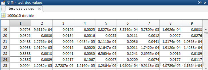
dec_values，一个矩阵包含决策的值或者概率估计。对于n个预测样本、k类的问题，如果指定“-b 1”参数，则n x k的矩阵，每一行表示这个样本分别属于每一个类别的概率；如果没有指定“-b 1”参数，则为n x k*(k-1)/2的矩阵，每一行表示k(k-1)/2个二分类SVM的预测结果；

test_label为测试样本标签，如果未知，可以随意给定，但必须和test_img_arr维数对应，如果已知，则在计算accuracy的时候，会将predict_label与test_label进行比较求准确度（对于多个测试样本）。

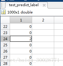
在svmtrain的时候设置’-b 1’，svmpredict的时候设置’-b 1’，可以看到dec_values的值为每一个样本属于每一个类别的概率，我们看下第24个测试样本，正确分类应该是数字0，即应该分到第一类，其dec_values值最大的是0.5217属于第三类，即数字2，与predict_label相吻合。

参考：

http://blog.sina.com.cn/s/blog_6646924501018fqc.html

http://blog.csdn.net/bryan__/article/details/51506801