


本次实践学习并练习使用R语言rpart包构建决策树,寻找决定高薪合同的技术统计元素。
期间用到了过采样方法解决目标样本量太少的问题,并应用了AUC、KS、混肴矩阵、精确度等模型评价指标,算是决策树的一次比较完备的实例实践。上代码:
#载入分析所需要的包
library(dplyr)
library(devtools)
library(woe)
library(ROSE)
library(rpart)
library(rpart.plot)
library(ggplot2)
require(caret)
library(pROC)
使用Rmarkdown写code时我喜欢把整个工程用到的包都在最开始的地方载入,可以设置(include=FALSE)不展示这部分代码,好处是通篇比较干净整洁。
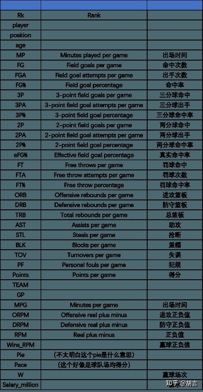
本文用到的数据依旧是为2016-2017赛季NBA300多为球员的技术统计,感谢简书用户“牧羊的男孩”,地址如下:
https://pan.baidu.com/s/1VjMGm9uzmeb5lnzPkGpD-Q
以下为“牧羊的男孩”提供的数据字段解释,非常感谢!
dat_nba<-read.csv('nba_2017_nba_players_with_salary.csv')
dat_nba$cut_salary<-ifelse(dat_nba$SALARY_MILLIONS>15,1,0)
dat_nba$cut_salary<-as.factor(dat_nba$cut_salary)
dat_nba<-select(dat_nba,-PLAYER,-SALARY_MILLIONS,-TEAM)
cat('目标变量:n')
summary(dat_nba$cut_salary)
cat('n')
names(dat_nba)
目标变量:
- 0 1
- 291 51
- [1] "X" "Rk" "POSITION" "AGE" "MP" "FG"
- [7] "FGA" "FG." "X3P" "X3PA" "X3P." "X2P"
- [13] "X2PA" "X2P." "eFG." "FT" "FTA" "FT."
- [19] "ORB" "DRB" "TRB" "AST" "STL" "BLK"
- [25] "TOV" "PF" "POINTS" "GP" "MPG" "ORPM"
- [31] "DRPM" "RPM" "WINS_RPM" "PIE" "PACE" "W"
计算IV值:
#install_github("riv","tomasgreif")
#library(devtools)
#library(woe)
IV<-iv.mult(dat_nba,"cut_salary",TRUE)   #原理是以Y作为被解释变量,其他作为解释变量,建立决策树模型
iv.plot.summary(IV)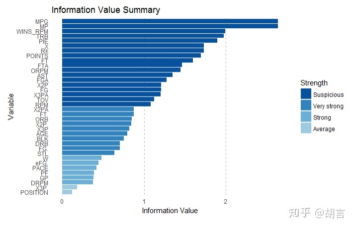
过采样方法:
#install.packages("ROSE")
#library(ROSE)
# 过采样&下采样
datt1<-dat_nba
table(datt1$cut_salary)
data_balanced_both <- ovun.sample(cut_salary ~ ., data = datt1, method = "both", p=0.5,N=342,seed = 1)$data
table(data_balanced_both$cut_salary)
原始样本正负比例:
- 0 1
- 291 51
过采样后正负比例:
- 0 1
- 183 159
#library(rpart)

#设置随机分配,查分数据为train集和test集#
dat=data_balanced_both
smp_size <- floor(0.6 * nrow(dat))
set.seed(123)
train_ind <- sample(seq_len(nrow(dat)), size = smp_size)
train <- dat[train_ind, ]
test <- dat[-train_ind, ]
dim(train)
dim(test)

fit<-(cut_salary~.)
rtree<-rpart(fit,minsplit=10, cp=0.03,data=train)
printcp(rtree)

#library(rpart.plot) #调出rpart.plot包
rpart.plot(rtree, type=2) 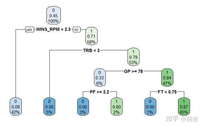
Warning message:
In strsplit(code, "n", fixed = TRUE) :
input string 1 is invalid in this locale
- [1] 205 37
- [1] 137 37
Classification tree:
rpart(formula = fit, data = train, minsplit = 10, cp = 0.03)
Variables actually used in tree construction:
[1] FT GP PF TRB WINS_RPM
Root node error: 93/205 = 0.45366
n= 205
CP nsplit rel error xerror xstd
- 1 0.548387 0 1.00000 1.00000 0.076646
- 2 0.118280 1 0.45161 0.50538 0.064717
- 3 0.043011 2 0.33333 0.40860 0.059826
- 4 0.032258 3 0.29032 0.34409 0.055878
- 5 0.030000 5 0.22581 0.33333 0.055156
#检验预测效果#
pre_train<-predict(rtree,type = 'vector') #type = c("vector", "prob", "class", "matrix"),
table(pre_train,train$cut_salary)

#检验test集预测效果#
pre_test<-predict(rtree, newdata = test,type = 'vector')
table(pre_test, test$cut_salary)

#检验整体集预测效果#
pre_dat<-predict(rtree, newdata = datt1,type = 'class')
table(pre_dat, datt1$cut_salary)
train集: 0 1
- 99 8
- 13 85
test集 0 1
- 60 13
- 11 53
pre_dat 0 1
- 237 10
- 54 41
评价决策树:
result=datt1
result$true_label=result$cut_salary
result$pre_prob=pre_dat
#install.packages("gmodels")
TPR <- NULL
FPR <- NULL
for(i in seq(from=1,to=0,by=-0.1)){
#判为正类实际也为正类
TP <- sum((result$pre_prob >= i) * (result$true_label == 1))
#判为正类实际为负类
FP <- sum((result$pre_prob >= i) * (result$true_label == 0))
#判为负类实际为负类
TN <- sum((result$pre_prob < i) * (result$true_label == 0))
#判为负类实际为正类
FN <- sum((result$pre_prob < i) * (result$true_label == 1))
TPR <- c(TPR,TP/(TP+FN))
FPR <- c(FPR,FP/(FP+TN))
}
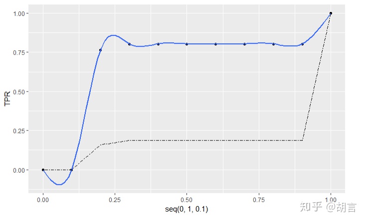
max(TPR-FPR) #KS
#library(ggplot2)
ggplot(data=NULL,mapping = aes(x=seq(0,1,0.1),y=TPR))+
geom_point()+
geom_smooth(se=FALSE,formula = y ~ splines::ns(x,10), method ='lm')+
geom_line(mapping = aes(x=seq(0,1,0.1),y=FPR),linetype=6)KS值为:
[1] 0.3277339
# 找到KS值对应的切分点:
for (i in seq(0,10,1)){
  print(i)
  print(TPR[i]-FPR[i])
}
## 混肴矩阵
result$pre_to1<-ifelse(result$pre_prob>=0.7,1,0)
#require(caret)
xtab<-table(result$pre_to1,result$true_label)
confusionMatrix(xtab)
[1] 0
numeric(0)
- [1] 1
- [1] 0
- [1] 2
- [1] 0
- [1] 3
- [1] 0.6066303
- [1] 4
- [1] 0.6183546
- [1] 5
- [1] 0.6183546
- [1] 6
- [1] 0.6183546
- [1] 7
- [1] 0.6183546
- [1] 8
- [1] 0.6183546
- [1] 9
- [1] 0.6183546
- [1] 10
- [1] 0.6183546
Confusion Matrix and Statistics
0 1
0 237 10
1 54 41
Accuracy : 0.8129
95% CI : (0.7674, 0.8528)
No Information Rate : 0.8509
P-Value [Acc > NIR] : 0.9772
Kappa : 0.4561
Mcnemar's Test P-Value : 7.658e-08
- Sensitivity : 0.8144
- Specificity : 0.8039
- Pos Pred Value : 0.9595
- Neg Pred Value : 0.4316
- Prevalence : 0.8509
- Detection Rate : 0.6930
- Detection Prevalence : 0.7222
- Balanced Accuracy : 0.8092
- 'Positive' Class : 0
## roc曲线及AUC
#library(pROC)
datt1_pro<-predict(rtree, newdata = datt1,type = 'prob')
datt1$pre_prob<-datt1_pro[,2]
modelroc <- roc(datt1$cut_salary,datt1$pre_prob)
plot(modelroc, print.auc=TRUE, auc.polygon=TRUE, grid=c(0.1, 0.2),
     grid.col=c("green", "red"), max.auc.polygon=TRUE,
     auc.polygon.col="skyblue", print.thres=TRUE)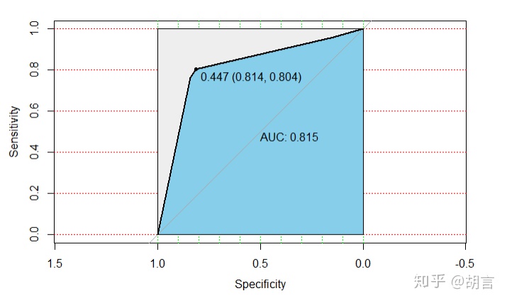
#设置随机分配,查分数据为train集和test集#
dat=datt1
smp_size <- floor(0.5 * nrow(dat))
train_ind <- sample(seq_len(nrow(dat)), size = smp_size)
train_2 <- dat[train_ind, ]
test_2 <- dat[-train_ind, ]
dim(train_2)
dim(test_2)
#检验预测效果#
pre_train_2<-predict(rtree,newdata=train_2,type = 'vector')
table(pre_train_2,train_2$cut_salary)
#检验test集预测效果#
pre_test_2<-predict(rtree, newdata = test_2,type = 'vector')
table(pre_test_2, test_2$cut_salary)
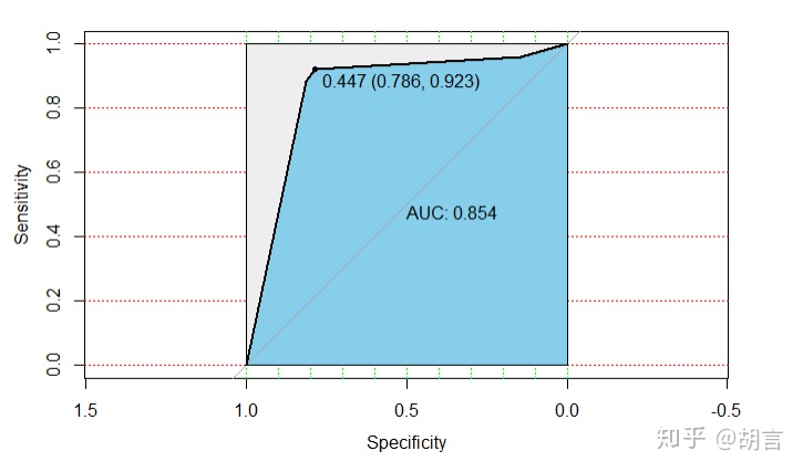
pre_train_2p<-predict(rtree,newdata=train_2,type = 'prob')
train_2$pre<-pre_train_2p[,2]
modelroc <- roc(train_2$cut_salary,train_2$pre)
plot(modelroc, print.auc=TRUE, auc.polygon=TRUE, grid=c(0.1, 0.2),
grid.col=c("green", "red"), max.auc.polygon=TRUE,
auc.polygon.col="skyblue", print.thres=TRUE)
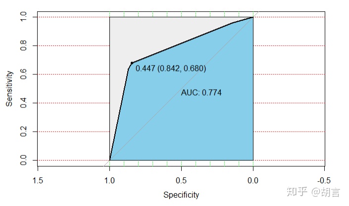
pre_test_2p<-predict(rtree, newdata = test_2,type = 'prob')
test_2$pre<-pre_test_2p[,2]
modelroc <- roc(test_2$cut_salary,test_2$pre)
plot(modelroc, print.auc=TRUE, auc.polygon=TRUE, grid=c(0.1, 0.2),
grid.col=c("green", "red"), max.auc.polygon=TRUE,
auc.polygon.col="skyblue", print.thres=TRUE)- [1] 171 38
- [1] 171 38
- pre_train_2 0 1
- 1 114 2
- 2 31 24
- pre_test_2 0 1
- 1 123 8
- 2 23 17


 8344
8344


 被折叠的 条评论
为什么被折叠?
被折叠的 条评论
为什么被折叠?
 到【灌水乐园】发言


