ls信道估计matlab_飞机参数辨识方法1——Equation-Error方法Matlab实例

（这是一篇学习笔记……）

1.方法原理

飞机参数辨识的Equation-error方法就是基于无量纲气动力和力矩系数与飞机状态和输入量的关系式，进行线性回归。

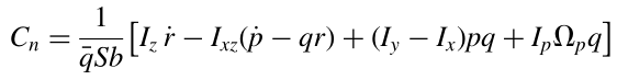
例如飞机航向力矩系数方程为：

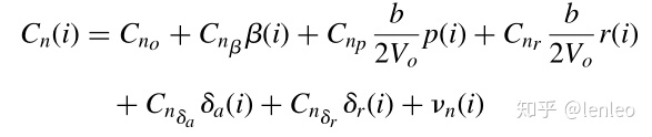
等式左边的航向力矩系数可以通过试验测得或通过角加速度数据推导出来，

等式右边的飞行参数包括侧滑角

，滚转角速度

，偏航角速度

，输入量包括副翼输入

，方向舵输入

，

是等效误差或噪声。为了估计

,

,

,

,

,

等气动导数，我们假设上述飞行参数和输入量都是可以

准确测得的，然后就可以利用线性回归进行估计了。

2. 参数辨识实例

下面使用matlab进行一个简单的示例。

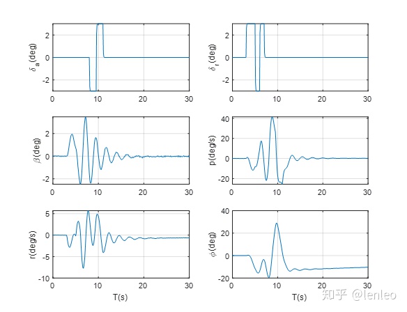
使用非线性F-16飞机模型进行仿真，考虑大气紊流（过程噪声）和传感器噪声（测量噪声），进行方向舵的“2-1-1”操纵和副翼的双向方波操纵，得到“试飞”数据。

% Equation error least square system identification

把所有回归项绘在一张图上，

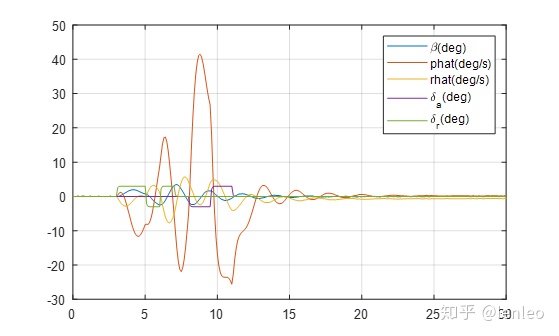
%% Assemble the regressor matrix
% beta p r da dr
X=[y_sim(:,9),y_sim(:,10),y_sim(:,12),surfaces(:,3),surfaces(:,4)];
% plot the regressor
figure(2)
plot(T,X,'LineWidth',1)
grid on
legend('beta(deg)','phat(deg/s)','rhat(deg/s)','delta_a(deg)','delta_r(deg)');

进行线性回归

%% LS process
% requires a constant regressor for the bias term
X=[X,ones(size(X,1),1)];
Cn = Coeff(:,5);
[yn,pn,crbn,s2n]=LS_fcn(X,Cn);
%      yn = model output vector.
%      pn = vector of parameter estimates.
%    crbn = estimated parameter covariance matrix.
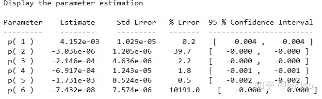
%     s2n = model fit error variance estimate.

回归结果，包括输出Cn的拟合结果和其他回归模型参数信息（估计值，标准差，百分误差，95%置信区间）

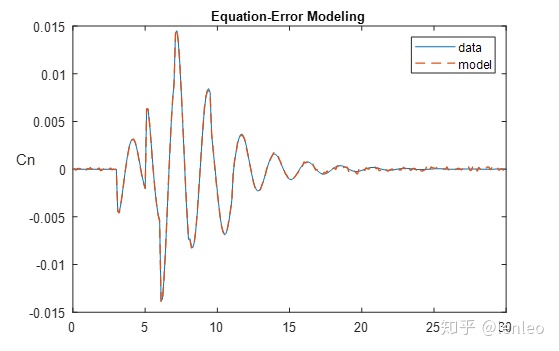
figure(3)
plot(T,Cn,T,yn,'--','LineWidth',1)
ylabel('Cn','Rotation',0);
title('Equation-Error Modeling','FontSize',10,'FontWeight','bold');
legend('data','model');
%% disp the result
fprintf('nn Display the parameter estimation ')
serrn=sqrt(diag(crbn));
xnames={'beta';'p';'r';'da';'dr'};
result_disp(pn,serrn,xnames);

残差分析，绘制残差-时间图和残差-输出图，可见绝大部分残差位于95%预测置信区间。

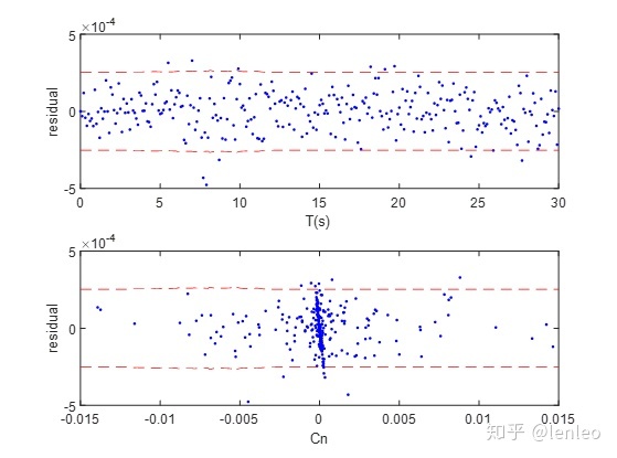
figure(4)
subplot(2,1,1),plot(T,Cn-yn,'b.'),grid on, hold on,
%  Prediction interval calculation.
[syn,yln]=confin_interv(X,pn,s2n);
%  Plot the 95 percent confidence interval for prediction.
plot(T,yln(:,1)-yn,'r--'),
plot(T,yln(:,2)-yn,'r--'),
hold off,
grid off,
ylabel('residual')
xlabel('T(s)')

subplot(2,1,2),plot(yn,Cn-yn,'b.'),grid on, hold on,
npts=length(yn);
plot([-0.015:0.03/(npts-1):0.015]',yln(:,1)-yn,'r--'),
plot([-0.015:0.03/(npts-1):0.015]',yln(:,2)-yn,'r--'),
hold off,
grid off,
ylabel('residual')
xlabel('Cn')

模型预测能力评估。选取另一段“试飞数据”，用刚刚得到的回归模型进行预测并和实际输出做对比，结果表明回归模型预测能力很好。

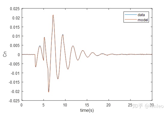
load F16_lat_w_vnoise2
XP = [y_sim(:,9),y_sim(:,10),y_sim(:,12),surfaces(:,3),surfaces(:,4)];
XP = [XP,ones(size(XP,1),1)];
CnP = Coeff(:,5);
ynP = XP*pn;
figure(6)
plot(T,CnP,T,ynP,'LineWidth',1);
legend('data','model');
xlabel('time(s)')
ylabel('Cn')

存在问题：

1. 实际上测量误差可能比较大，仿真数据难以体现真实情况
2. 风洞试验中可以直接测出气动力和力矩系数，飞行试验数据中没有，只能通过其他数据推算，引入了不确定性
3. 假设残差是白噪声，但实际上是有色噪声，这个冲突虽不影响估计值期望，但影响方差，需要对方差进行校正。
4. 需要已知模型，实际上有很多项影响较小，需要做model reduction。

附上上述代码和数据

https://github.com/lenleo1/Aircraft_parameter_estimation/tree/main/01Error_Equation​github.com

参考文献：

[1]Russell R S. Non-linear F-16 simulation using Simulink and Matlab[J]. University of Minnesota, Tech. paper, 2003.

[2]Morelli E A, Klein V. Aircraft system identification: theory and practice[M]. Williamsburg, VA: Sunflyte Enterprises, 2016.