


♥
ex7.m
%% Machine Learning Online Class% Exercise 7 | Principle Component Analysis and K-Means Clustering%% Instructions% ------------%% This file contains code that helps you get started on the% exercise. You will need to complete the following functions:%% pca.m% projectData.m% recoverData.m% computeCentroids.m% findClosestCentroids.m% kMeansInitCentroids.m%% For this exercise, you will not need to change any code in this file,% or any other files other than those mentioned above.%%% Initializationclear ; close all; clc%% ================= Part 1: Find Closest Centroids ====================% To help you implement K-Means, we have divided the learning algorithm % into two functions -- findClosestCentroids and computeCentroids. In this% part, you should complete the code in the findClosestCentroids function. %fprintf('Finding closest centroids.\n\n');% Load an example dataset that we will be usingload('ex7data2.mat');% Select an initial set of centroidsK = 3; % 3 Centroidsinitial_centroids = [3 3; 6 2; 8 5];% Find the closest centroids for the examples using the% initial_centroidsidx = findClosestCentroids(X, initial_centroids);fprintf('Closest centroids for the first 3 examples: \n')fprintf(' %d', idx(1:3));fprintf('\n(the closest centroids should be 1, 3, 2 respectively)\n');fprintf('Program paused. Press enter to continue.\n');pause;%% ===================== Part 2: Compute Means =========================% After implementing the closest centroids function, you should now% complete the computeCentroids function.%fprintf('\nComputing centroids means.\n\n');% Compute means based on the closest centroids found in the previous part.centroids = computeCentroids(X, idx, K);fprintf('Centroids computed after initial finding of closest centroids: \n')fprintf(' %f %f \n' , centroids');fprintf('\n(the centroids should be\n');fprintf(' [ 2.428301 3.157924 ]\n');fprintf(' [ 5.813503 2.633656 ]\n');fprintf(' [ 7.119387 3.616684 ]\n\n');fprintf('Program paused. Press enter to continue.\n');pause;%% =================== Part 3: K-Means Clustering ======================% After you have completed the two functions computeCentroids and% findClosestCentroids, you have all the necessary pieces to run the% kMeans algorithm. In this part, you will run the K-Means algorithm on% the example dataset we have provided. %fprintf('\nRunning K-Means clustering on example dataset.\n\n');% Load an example datasetload('ex7data2.mat');% Settings for running K-MeansK = 3;max_iters = 10;% For consistency, here we set centroids to specific values% but in practice you want to generate them automatically, such as by% settings them to be random examples (as can be seen in% kMeansInitCentroids).initial_centroids = [3 3; 6 2; 8 5];% Run K-Means algorithm. The 'true' at the end tells our function to plot% the progress of K-Means[centroids, idx] = runkMeans(X, initial_centroids, max_iters, true);fprintf('\nK-Means Done.\n\n');fprintf('Program paused. Press enter to continue.\n');pause;%% ============= Part 4: K-Means Clustering on Pixels ===============% In this exercise, you will use K-Means to compress an image. To do this,% you will first run K-Means on the colors of the pixels in the image and% then you will map each pixel onto its closest centroid.% % You should now complete the code in kMeansInitCentroids.m%fprintf('\nRunning K-Means clustering on pixels from an image.\n\n');% Load an image of a birdA = double(imread('bird_small.png'));% If imread does not work for you, you can try instead% load ('bird_small.mat');A = A / 255; % Divide by 255 so that all values are in the range 0 - 1% Size of the imageimg_size = size(A);% Reshape the image into an Nx3 matrix where N = number of pixels.% Each row will contain the Red, Green and Blue pixel values% This gives us our dataset matrix X that we will use K-Means on.X = reshape(A, img_size(1) * img_size(2), 3);% Run your K-Means algorithm on this data% You should try different values of K and max_iters hereK = 16; max_iters = 10;% When using K-Means, it is important the initialize the centroids% randomly. % You should complete the code in kMeansInitCentroids.m before proceedinginitial_centroids = kMeansInitCentroids(X, K);% Run K-Means[centroids, idx] = runkMeans(X, initial_centroids, max_iters);fprintf('Program paused. Press enter to continue.\n');pause;%% ================= Part 5: Image Compression ======================% In this part of the exercise, you will use the clusters of K-Means to% compress an image. To do this, we first find the closest clusters for% each example. After that, we fprintf('\nApplying K-Means to compress an image.\n\n');% Find closest cluster membersidx = findClosestCentroids(X, centroids);% Essentially, now we have represented the image X as in terms of the% indices in idx. % We can now recover the image from the indices (idx) by mapping each pixel% (specified by its index in idx) to the centroid valueX_recovered = centroids(idx,:);% Reshape the recovered image into proper dimensionsX_recovered = reshape(X_recovered, img_size(1), img_size(2), 3);% Display the original image subplot(1, 2, 1);imagesc(A); title('Original');% Display compressed image side by sidesubplot(1, 2, 2);imagesc(X_recovered)title(sprintf('Compressed, with %d colors.', K));fprintf('Program paused. Press enter to continue.\n');pause;ex7_pca.m
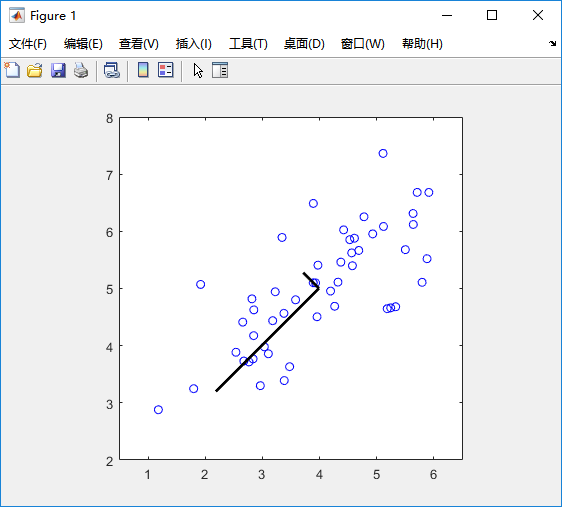
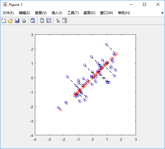
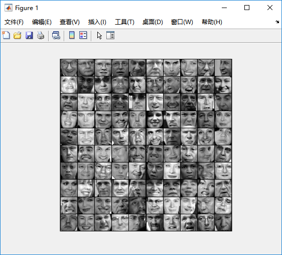
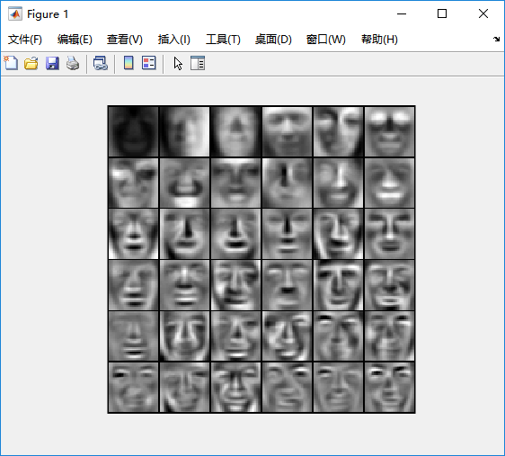
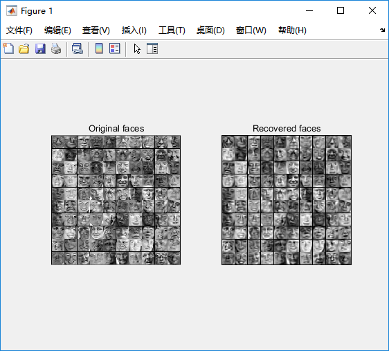
%% Machine Learning Online Class% Exercise 7 | Principle Component Analysis and K-Means Clustering%% Instructions% ------------%% This file contains code that helps you get started on the% exercise. You will need to complete the following functions:%% pca.m% projectData.m% recoverData.m% computeCentroids.m% findClosestCentroids.m% kMeansInitCentroids.m%% For this exercise, you will not need to change any code in this file,% or any other files other than those mentioned above.%%% Initializationclear ; close all; clc%% ================== Part 1: Load Example Dataset ===================% We start this exercise by using a small dataset that is easily to% visualize%fprintf('Visualizing example dataset for PCA.\n\n');% The following command loads the dataset. You should now have the % variable X in your environmentload ('ex7data1.mat');% Visualize the example datasetplot(X(:, 1), X(:, 2), 'bo');axis([0.5 6.5 2 8]); axis square;fprintf('Program paused. Press enter to continue.\n');pause;%% =============== Part 2: Principal Component Analysis ===============% You should now implement PCA, a dimension reduction technique. You% should complete the code in pca.m%fprintf('\nRunning PCA on example dataset.\n\n');% Before running PCA, it is important to first normalize X[X_norm, mu, sigma] = featureNormalize(X);% Run PCA[U, S] = pca(X_norm);% Compute mu, the mean of the each feature% Draw the eigenvectors centered at mean of data. These lines show the% directions of maximum variations in the dataset.hold on;drawLine(mu, mu + 1.5 * S(1,1) * U(:,1)', '-k', 'LineWidth', 2);drawLine(mu, mu + 1.5 * S(2,2) * U(:,2)', '-k', 'LineWidth', 2);hold off;fprintf('Top eigenvector: \n');fprintf(' U(:,1) = %f %f \n', U(1,1), U(2,1));fprintf('\n(you should expect to see -0.707107 -0.707107)\n');fprintf('Program paused. Press enter to continue.\n');pause;%% =================== Part 3: Dimension Reduction ===================% You should now implement the projection step to map the data onto the % first k eigenvectors. The code will then plot the data in this reduced % dimensional space. This will show you what the data looks like when % using only the corresponding eigenvectors to reconstruct it.%% You should complete the code in projectData.m%fprintf('\nDimension reduction on example dataset.\n\n');% Plot the normalized dataset (returned from pca)plot(X_norm(:, 1), X_norm(:, 2), 'bo');axis([-4 3 -4 3]); axis square% Project the data onto K = 1 dimensionK = 1;Z = projectData(X_norm, U, K);fprintf('Projection of the first example: %f\n', Z(1));fprintf('\n(this value should be about 1.481274)\n\n');X_rec = recoverData(Z, U, K);fprintf('Approximation of the first example: %f %f\n', X_rec(1, 1), X_rec(1, 2));fprintf('\n(this value should be about -1.047419 -1.047419)\n\n');% Draw lines connecting the projected points to the original pointshold on;plot(X_rec(:, 1), X_rec(:, 2), 'ro');for i = 1:size(X_norm, 1) drawLine(X_norm(i,:), X_rec(i,:), '--k', 'LineWidth', 1);endhold offfprintf('Program paused. Press enter to continue.\n');pause;%% =============== Part 4: Loading and Visualizing Face Data =============% We start the exercise by first loading and visualizing the dataset.% The following code will load the dataset into your environment%fprintf('\nLoading face dataset.\n\n');% Load Face datasetload ('ex7faces.mat')% Display the first 100 faces in the datasetdisplayData(X(1:100, :));fprintf('Program paused. Press enter to continue.\n');pause;%% =========== Part 5: PCA on Face Data: Eigenfaces ===================% Run PCA and visualize the eigenvectors which are in this case eigenfaces% We display the first 36 eigenfaces.%fprintf(['\nRunning PCA on face dataset.\n' ... '(this might take a minute or two ...)\n\n']);% Before running PCA, it is important to first normalize X by subtracting % the mean value from each feature[X_norm, mu, sigma] = featureNormalize(X);% Run PCA[U, S] = pca(X_norm);% Visualize the top 36 eigenvectors founddisplayData(U(:, 1:36)');fprintf('Program paused. Press enter to continue.\n');pause;%% ============= Part 6: Dimension Reduction for Faces =================% Project images to the eigen space using the top k eigenvectors % If you are applying a machine learning algorithm fprintf('\nDimension reduction for face dataset.\n\n');K = 100;Z = projectData(X_norm, U, K);fprintf('The projected data Z has a size of: ')fprintf('%d ', size(Z));fprintf('\n\nProgram paused. Press enter to continue.\n');pause;%% ==== Part 7: Visualization of Faces after PCA Dimension Reduction ====% Project images to the eigen space using the top K eigen vectors and % visualize only using those K dimensions% Compare to the original input, which is also displayedfprintf('\nVisualizing the projected (reduced dimension) faces.\n\n');K = 100;X_rec = recoverData(Z, U, K);% Display normalized datasubplot(1, 2, 1);displayData(X_norm(1:100,:));title('Original faces');axis square;% Display reconstructed data from only k eigenfacessubplot(1, 2, 2);displayData(X_rec(1:100,:));title('Recovered faces');axis square;fprintf('Program paused. Press enter to continue.\n');pause;%% === Part 8(a): Optional (ungraded) Exercise: PCA for Visualization ===% One useful application of PCA is to use it to visualize high-dimensional% data. In the last K-Means exercise you ran K-Means on 3-dimensional % pixel colors of an image. We first visualize this output in 3D, and then% apply PCA to obtain a visualization in 2D.close all; close all; clc% Reload the image from the previous exercise and run K-Means on it% For this to work, you need to complete the K-Means assignment firstA = double(imread('bird_small.png'));% If imread does not work for you, you can try instead% load ('bird_small.mat');A = A / 255;img_size = size(A);X = reshape(A, img_size(1) * img_size(2), 3);K = 16; max_iters = 10;initial_centroids = kMeansInitCentroids(X, K);[centroids, idx] = runkMeans(X, initial_centroids, max_iters);% Sample 1000 random indexes (since working with all the data is% too expensive. If you have a fast computer, you may increase this.sel = floor(rand(1000, 1) * size(X, 1)) + 1;% Setup Color Palettepalette = hsv(K);colors = palette(idx(sel), :);% Visualize the data and centroid memberships in 3Dfigure;scatter3(X(sel, 1), X(sel, 2), X(sel, 3), 10, colors);title('Pixel dataset plotted in 3D. Color shows centroid memberships');fprintf('Program paused. Press enter to continue.\n');pause;%% === Part 8(b): Optional (ungraded) Exercise: PCA for Visualization ===% Use PCA to project this cloud to 2D for visualization% Subtract the mean to use PCA[X_norm, mu, sigma] = featureNormalize(X);% PCA and project the data to 2D[U, S] = pca(X_norm);Z = projectData(X_norm, U, 2);% Plot in 2Dfigure;plotDataPoints(Z(sel, :), idx(sel), K);title('Pixel dataset plotted in 2D, using PCA for dimensionality reduction');fprintf('Program paused. Press enter to continue.\n');pause;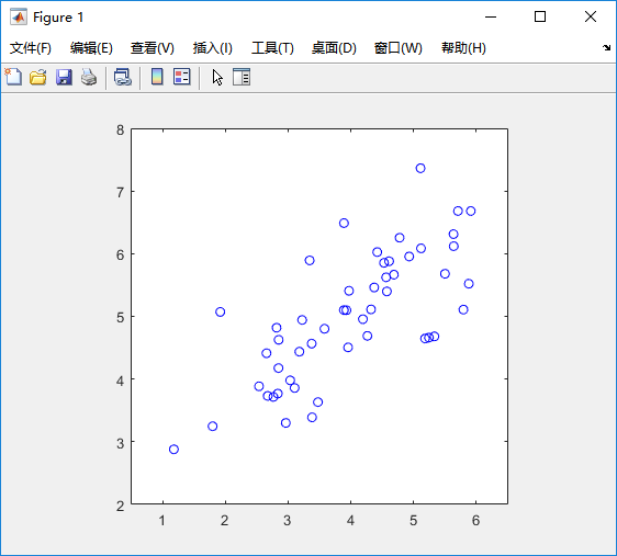


 6883
6883


 被折叠的 条评论
为什么被折叠?
被折叠的 条评论
为什么被折叠?
 到【灌水乐园】发言


