python standardscaler_python主成分分析小实例

原文地址

Principal Component Analysis (PCA) with Python

导入需要的模块

import matplotlib.pyplot as plt
import pandas as pd
import seaborn as sns
import numpy as np
from sklearn.preprocessing import StandardScaler
from sklearn.decomposition import PCA

读入数据

数据获取连接 https://archive.ics.uci.edu/ml/machine-learning-databases/iris/iris.data

df = pd.read_csv("Desktop/Python_GUI/Tkinter/iris.csv")
df.head()
Out[8]: 
   sepal length  sepal width  petal lenght  petal width       target
0           5.1          3.5           1.4          0.2  Iris-setosa
1           4.9          3.0           1.4          0.2  Iris-setosa
2           4.7          3.2           1.3          0.2  Iris-setosa
3           4.6          3.1           1.5          0.2  Iris-setosa
4           5.0          3.6           1.4          0.2  Iris-setosa

主成分分析

df1 = df.loc[:,df.columns[0:4]]
scaler = StandardScaler()
scaler.fit(df1)
scaled_df = scaler.transform(df1)
pca = PCA(n_components = 4)
pca.fit(scaled_df)
x_pca = pca.transform(scaled_df)
pca.explained_variance_ratio_
plt.bar(x = range(1,5),height=percent_variance,tick_label=["PC" + str(i) for i in range(1,5)])
plt.ylabel('Percentate of Variance Explained')
plt.xlabel('Principal Component')
plt.title('PCA Scree Plot')
plt.savefig("1.jpg")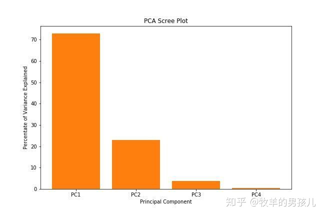

df2 = pd.DataFrame(data=x_pca,columns=["PC"+str(i) for i in range(1,5)])
df3 = pd.concat([df2,df['target']],axis=1)
plt.figure(figsize=(9,6))
sns.scatterplot(x="PC1",y="PC2",hue='target',data=df3)
plt.xlabel("PC1")
plt.ylabel("PC2")
plt.title("PC1 VS PC2")
plt.savefig("2.jpg")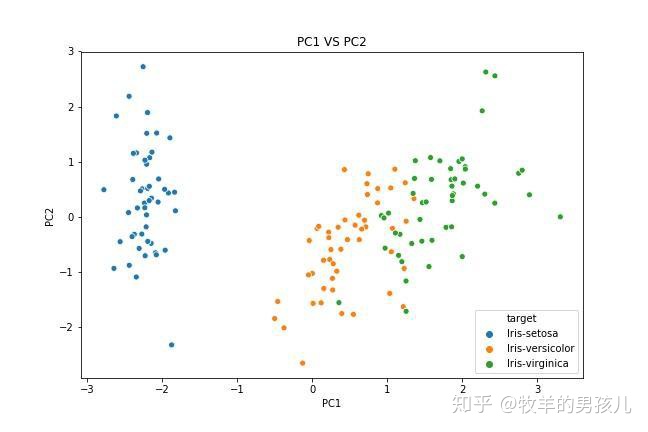

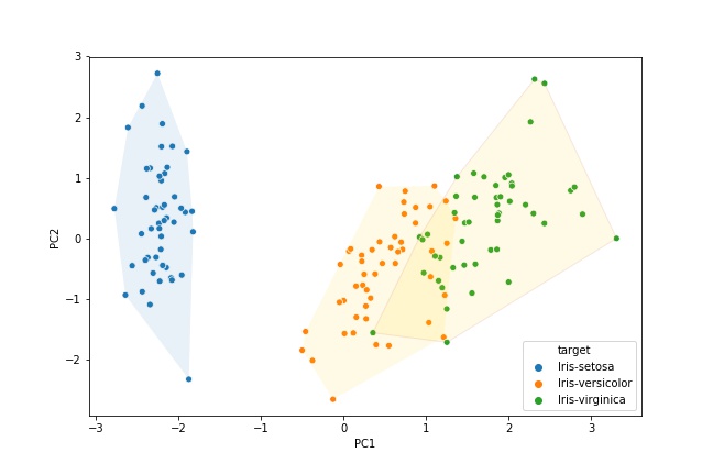
为不同的品种绘制边界

代码来自知乎文章 数据分析最有用的25个 Matplotlib图（一） 用到的代码自己还看不懂

from matplotlib import patches
from scipy.spatial import ConvexHull
#这个函数的代码自己还看不懂
def encircle(x,y, ax=None, **kw):
    if not ax: ax=plt.gca()
    p = np.c_[x,y]
    hull = ConvexHull(p)
    poly = plt.Polygon(p[hull.vertices,:], **kw)
    ax.add_patch(poly)
df3_1 = df3.loc[df3.target == df3.target.unique()[0],:]
df3_2 = df3.loc[df3.target == df3.target.unique()[1],:]
df3_3 = df3.loc[df3.target == df3.target.unique()[2],:]
plt.figure(figsize=(9,6))
sns.scatterplot(x="PC1",y="PC2",hue='target',data=df3)
encircle(df3_1.PC1,df3_1.PC2,alpha=0.1)
encircle(df3_2.PC1,df3_2.PC2,fc = "gold", alpha=0.1)
encircle(df3_3.PC1,df3_3.PC2,ec = "firebrick",fc = "gold", alpha=0.1)
plt.savefig("3.jpg")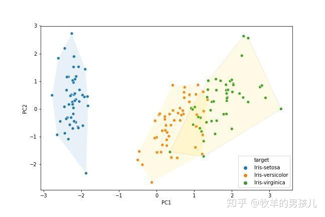

参考文章

• https://datascienceplus.com/principal-component-analysis-pca-with-python/
• https://scikit-learn.org/stable/auto_examples/decomposition/plot_pca_iris.html
• https://www.jianshu.com/p/4528aaa6dc48
• https://scikit-learn.org/stable/auto_examples/decomposition/plot_pca_iris.html
• https://www.kindsonthegenius.com/2019/01/12/principal-components-analysispca-in-python-step-by-step/
• https://jakevdp.github.io/PythonDataScienceHandbook/05.09-principal-component-analysis.html