数学建模最小二乘法拟合_MATLAB最小二乘法拟合曲线公式

假设 y = f(x)，那么每个x应该会对应一个y。对一个未知公式的 f(x)系统，在科学实验中，常常需要测量两个变量的多组数据，然后找出他们的近似函数关系。通常，我们把这种处理数据的方法称之为经验配线，所找到的函数关系称为经验公式。最小二乘法就是最常用的一种配线方式。

最小二乘法是一种数学优化技术，它通过最小误差的平方和找到一组数据的最佳函数匹配。最小二乘法常用于曲线拟合。

下面，我们通过一个例子来研究最小二乘法函数polyfit的使用。

首先，我们通过数据采集，得到一组y和x数据的对应关系并绘制成曲线。

x = [88    88    96    98    99   101   101   102   102   104   105   106   107   109   111   113   113   113   116   119   121   121   126   128   128   132   134   140   140   141   141  145   147   148  150   153   154   154   154   155   158   160   161   165   166   168   172   174];

y = [2.5882       2.7059       2.8729       2.8834       2.9814       3.0909       3.1638       3.2353       3.3929       3.5404       3.6158       3.7569       3.8235        3.865   3.8824       3.9286       3.9394       4.1765       4.2353       4.3558       4.5856       4.6061       4.6584       4.7059       4.7826       4.8066       4.8214       4.8824   4.9697       5.0847        5.092        5.092       5.1381       5.1553       5.1786       5.2381       5.2727       5.4118       5.4237       5.5882       5.5932       5.8564   5.9627        6.135       6.4972       6.6071       6.6471       6.8485];

plot(x,y,'o');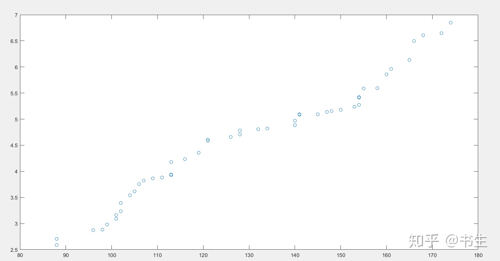

原始采样数据

通过polyfit进行一阶拟合

x = [88    88    96    98    99   101   101   102   102   104   105   106   107   109   111   113   113   113   116   119   121   121   126   128   128   132   134   140   140   141   141  145   147   148  150   153   154   154   154   155   158   160   161   165   166   168   172   174];

y = [2.5882       2.7059       2.8729       2.8834       2.9814       3.0909       3.1638       3.2353       3.3929       3.5404       3.6158       3.7569       3.8235        3.865   3.8824       3.9286       3.9394       4.1765       4.2353       4.3558       4.5856       4.6061       4.6584       4.7059       4.7826       4.8066       4.8214       4.8824   4.9697       5.0847        5.092        5.092       5.1381       5.1553       5.1786       5.2381       5.2727       5.4118       5.4237       5.5882       5.5932       5.8564   5.9627        6.135       6.4972       6.6071       6.6471       6.8485];

%一阶拟合
coefficient=polyfit(x,y,1);

%将拟合后系数带入公式 Y = P(1)*X^N + P(2)*X^(N-1) + ... + P(N)*X + P(N+1)
yn=polyval(coefficient,x);

plot(x,y,'o');hold on;
plot(x,yn,'-k');hold on;
legend(sprintf("x-y"),sprintf("yn = (%f)x + (%f)",coefficient(1,1),coefficient(1,2)));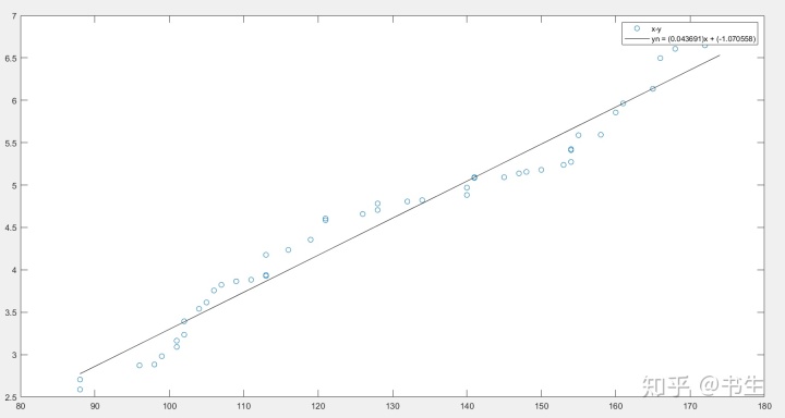

1阶拟合的曲线效果

通过polyfit进行二阶拟合

x = [88    88    96    98    99   101   101   102   102   104   105   106   107   109   111   113   113   113   116   119   121   121   126   128   128   132   134   140   140   141   141  145   147   148  150   153   154   154   154   155   158   160   161   165   166   168   172   174];

y = [2.5882       2.7059       2.8729       2.8834       2.9814       3.0909       3.1638       3.2353       3.3929       3.5404       3.6158       3.7569       3.8235        3.865   3.8824       3.9286       3.9394       4.1765       4.2353       4.3558       4.5856       4.6061       4.6584       4.7059       4.7826       4.8066       4.8214       4.8824   4.9697       5.0847        5.092        5.092       5.1381       5.1553       5.1786       5.2381       5.2727       5.4118       5.4237       5.5882       5.5932       5.8564   5.9627        6.135       6.4972       6.6071       6.6471       6.8485];

%二阶拟合
coefficient=polyfit(x,y,2);

%将拟合后系数带入公式 Y = P(1)*X^N + P(2)*X^(N-1) + ... + P(N)*X + P(N+1)
yn=polyval(coefficient,x);

plot(x,y,'o');hold on;
plot(x,yn,'-k');hold on;
legend(sprintf("x-y"),sprintf("yn = (%f)x² + (%f)x + (%f)",coefficient(1,1),coefficient(1,2),coefficient(1,3)));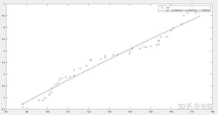

同理，可得到更多阶拟合的效果

3阶拟合

6阶拟合

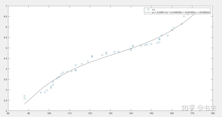
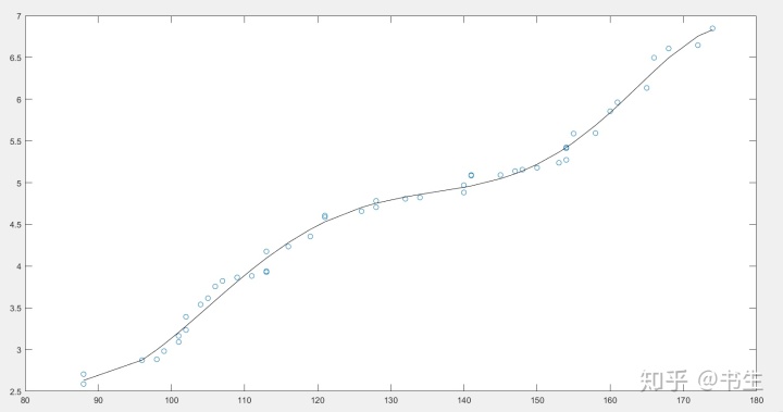
由此可见，在系统允许的条件下，阶数越多，拟合出来的曲线越逼近真实的测量曲线。这个工作要是放在人工设计里实现，将会是一个非常繁琐的事情，最小二乘法恰恰非常适合解决这类曲线拟合的工作。