


因果推理综述——《A Survey on Causal Inference》一文的总结和梳理
基础理论
理论框架
名词解释
- individual treatment effect :ITE = Y 1 i − Y 0 i Y_{1i}-Y_{0i} Y1i−Y0i
- average treatment effect :ATE= E ( Y 1 i − Y 0 i ) E(Y_{1i}-Y_{0i}) E(Y1i−Y0i)
- conditional treatment effect :CAPE = E ( Y 1 i − Y 0 i ∣ X ) E(Y_{1i}-Y_{0i}|X) E(Y1i−Y0i∣X)
两个挑战
- counterfact:无法观测到反事实数据
- confounder bias:treatment不是随机分配
1 Rubin Causal Model(RCM)
potential outcome model (虚拟事实模型 ),也叫做Rubin Causal Model(RCM),希望估计出每个unit或者整体平均意义下的potential outcome,进而得到干预效果treatment effect(eg. ITE/ATE)。
因此准确地估计出potential outcome是该框架的关键,由于混杂因子confounder的存在,观察到的数据不用直接用来近似potential outcome,需要有进一步的处理。
核心思想:准确估计potential outcome,寻找对照组
- matching:根据倾向得分,找到最佳对照组
- weighting/pairing:重加权
- subclassification/stratification:分层,求得CATE
2 Pearl Causal Graph(SCM)
通过计算因果图中的条件分布,获得变量之间的因果关系。有向图指导我们使用这些条件分布来消除估计偏差,其核心也是估计检验分布、消除其他变量带来的偏差。
- 链式结构:常见在前门路径,A -> C一定需要经过B
- 叉式结构:中间节点B通常被视为A和C的共因(common cause)或混杂因子(confounder )。混杂因子会使A和C在统计学上发生关联,即使它们没有直接的关系。经典例子:“鞋的尺码←孩子的年龄→阅读能力”,穿较大码的鞋的孩子年龄可能更大,所以往往有着更强的阅读能力,但当固定了年龄之后,A和C就条件独立了。
- 对撞结构:AB、BC相关,AC不相关;给定B时,AC相关
三个假设
1. 无混淆性(Unconfoundedness)
也称之为「条件独立性假设」(conditional independence assumption, CIA),即解决X->T的路径。
Given the background variable, X, treatment assignment T is independent to the potential outcomes Y
( Y 1 , Y 0 ) ⊥ W ∣ X (Y_1, Y_0) \perp W | X (Y1,Y0)⊥W∣X
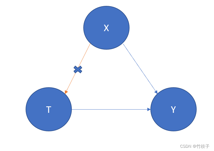
该假设使得具有相同X的unit是随机分配的。
2. 正值(Positivity)
For any value of X, treatment assignment is not deterministic
P ( W = w ∣ X = x ) > 0 P(W=w \mid X=x)>0 P(W=w∣X=x)>0
干预一定要有实验样本;干预、混杂因子越多,所需的样本也越多
3. 一致性(Consistency)
也可以叫「稳定单元干预值假设」(Stable Unit Treatment Value Assumption, SUTVA)
The potential outcomes for any unit do not vary with the treatment assigned to other units, and, for each unit, there are no different forms or versions of each treatment level, which lead to different potential outcomes.
任意单元的潜在结果都不会因其他单元的干预发生改变而改变,且对于每个单元,其所接受的每种干预不存在不同的形式或版本,不会导致不同的潜在结果。
混淆因素
Confounders are the variables that affect both the treatment assignment and the outcome.
Confounder大多会引起伪效应(spurious effect)和选择偏差(selection bias)。
-
针对spurious effect,根据X分布进行权重加和
ATE = ∑ x p ( x ) E [ Y F ∣ X = x , W = 1 ] − ∑ x p ( x ) E [ Y F ∣ X = x , W = 0 ] \text { ATE }=\sum_x p(x) \mathbb{E}\left[Y^F\mid X=x, W=1\right]-\sum_x p(x) \mathbb{E}\left[Y^F \mid X=x, W=0\right] ATE =x∑p(x)E[YF∣X=x,W=1]−x∑p(x)E[YF∣X=x,W=0] -
针对selection bias,为每个group找到对应的pseudo group,如sample re-weighting, matching, tree-based methods, confounder balancing, balanced representation learning methods, multi-task-based methods
建模方法
1. re-weighting methods*
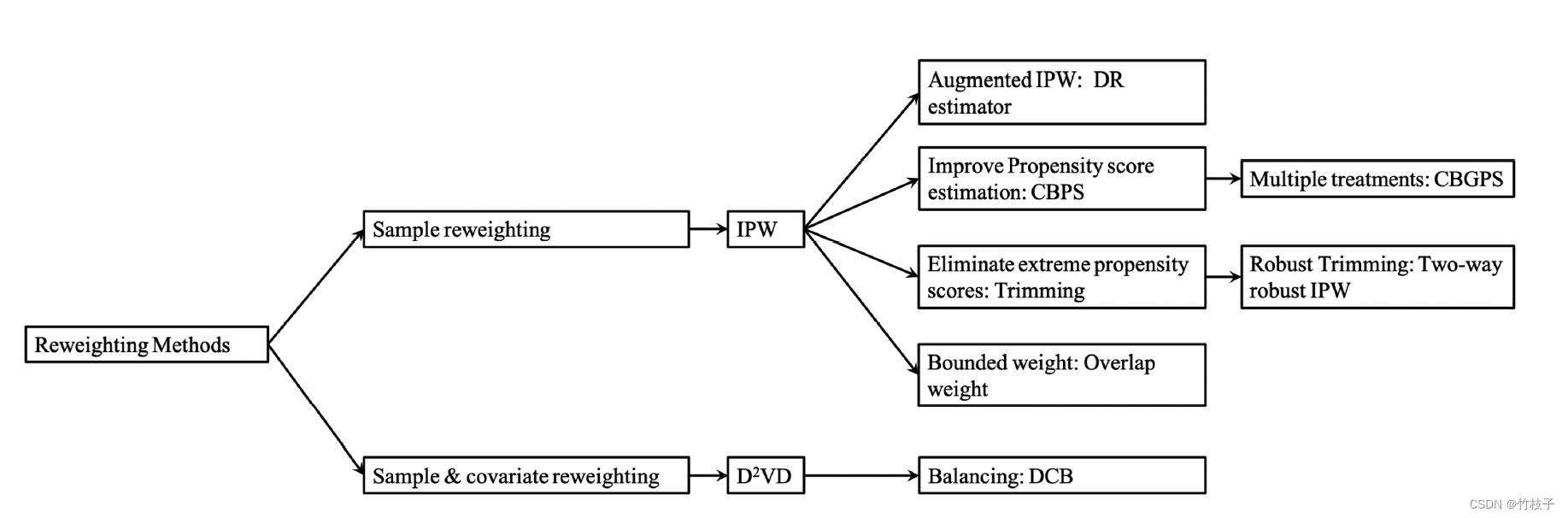
By assigning appropriate weight to each unit in the observational data, a pseudo-population can be created on which the distributions of the treated group and control group are similar.
通过给每个观测数据分配权重,调整treatment和control两个组的分布,使其接近。关键在于怎么选择balancing score,propensity score是特殊情况。
e ( x ) = Pr ( W = 1 ∣ X = x ) e(x)=\operatorname{Pr}(W=1 \mid X=x) e(x)=Pr(W=1∣X=x)
The propensity score can be used to balance the covariates in the treatment and control groups and therefore reduce the bias through matching, stratification (subclassification), regression adjustment, or some combination of all three.
1. Propensity Score Based Sample Re-weighting
IPW :
r
=
W
e
(
x
)
+
1
−
W
1
−
e
(
x
)
r=\frac{W}{e(x)}+\frac{1-W}{1-e(x)}
r=e(x)W+1−e(x)1−W,用r给每个样本算权重
A
T
E
I
P
W
=
1
n
∑
i
=
1
n
W
i
Y
i
F
e
^
(
x
i
)
−
1
n
∑
i
=
1
n
(
1
−
W
i
)
Y
i
F
1
−
e
^
(
x
i
)
\mathrm{ATE}_{I P W}=\frac{1}{n} \sum_{i=1}^n \frac{W_i Y_i^F}{\hat{e}\left(x_i\right)}-\frac{1}{n} \sum_{i=1}^n \frac{\left(1-W_i\right) Y_i^F}{1-\hat{e}\left(x_i\right)}
ATEIPW=n1i=1∑ne^(xi)WiYiF−n1i=1∑n1−e^(xi)(1−Wi)YiF
经normalization,
A
T
E
I
P
W
=
∑
i
=
1
n
W
i
Y
i
F
e
^
(
x
i
)
/
∑
i
=
1
n
W
i
e
^
(
x
i
)
−
∑
i
=
1
n
(
1
−
W
i
)
Y
i
F
1
−
e
^
(
x
i
)
/
∑
i
=
1
n
(
1
−
W
i
)
1
−
e
^
(
x
i
)
\mathrm{ATE}_{I P W}=\sum_{i=1}^n \frac{W_i Y_i^F}{\hat{e}\left(x_i\right)} / \sum_{i=1}^n \frac{W_i}{\hat{e}\left(x_i\right)}-\sum_{i=1}^n \frac{\left(1-W_i\right) Y_i^F}{1-\hat{e}\left(x_i\right)} / \sum_{i=1}^n \frac{\left(1-W_i\right)}{1-\hat{e}\left(x_i\right)}
ATEIPW=i=1∑ne^(xi)WiYiF/i=1∑ne^(xi)Wi−i=1∑n1−e^(xi)(1−Wi)YiF/i=1∑n1−e^(xi)(1−Wi)
缺点:极大依赖e(X)估计的准确性
DR:解决propensity score估计不准的问题
A
T
E
D
R
=
1
n
∑
i
=
1
n
{
[
W
i
Y
i
F
e
^
(
x
i
)
−
W
i
−
e
^
(
x
i
)
e
^
(
x
i
)
m
^
(
1
,
x
i
)
]
−
[
(
1
−
W
i
)
Y
i
F
1
−
e
^
(
x
i
)
−
W
i
−
e
^
(
x
i
)
1
−
e
^
(
x
i
)
m
^
(
0
,
x
i
)
]
}
=
1
n
∑
i
=
1
n
{
m
^
(
1
,
x
i
)
+
W
i
(
Y
i
F
−
m
^
(
1
,
x
i
)
)
e
^
(
x
i
)
−
m
^
(
0
,
x
i
)
−
(
1
−
W
i
)
(
Y
i
F
−
m
^
(
0
,
x
i
)
)
1
−
e
^
(
x
i
)
}
\begin{aligned} \mathrm{ATE}_{D R} &=\frac{1}{n} \sum_{i=1}^n\left\{\left[\frac{W_i Y_i^F}{\hat{e}\left(x_i\right)}-\frac{W_i-\hat{e}\left(x_i\right)}{\hat{e}\left(x_i\right)} \hat{m}\left(1, x_i\right)\right]-\left[\frac{\left(1-W_i\right) Y_i^F}{1-\hat{e}\left(x_i\right)}-\frac{W_i-\hat{e}\left(x_i\right)}{1-\hat{e}\left(x_i\right)} \hat{m}\left(0, x_i\right)\right]\right\} \\ &=\frac{1}{n} \sum_{i=1}^n\left\{\hat{m}\left(1, x_i\right)+\frac{W_i\left(Y_i^F-\hat{m}\left(1, x_i\right)\right)}{\hat{e}\left(x_i\right)}-\hat{m}\left(0, x_i\right)-\frac{\left(1-W_i\right)\left(Y_i^F-\hat{m}\left(0, x_i\right)\right)}{1-\hat{e}\left(x_i\right)}\right\} \end{aligned}
ATEDR=n1i=1∑n{[e^(xi)WiYiF−e^(xi)Wi−e^(xi)m^(1,xi)]−[1−e^(xi)(1−Wi)YiF−1−e^(xi)Wi−e^(xi)m^(0,xi)]}=n1i=1∑n{m^(1,xi)+e^(xi)Wi(YiF−m^(1,xi))−m^(0,xi)−1−e^(xi)(1−Wi)(YiF−m^(0,xi))}
m
^
(
1
,
x
i
)
\hat{m}\left(1, x_i\right)
m^(1,xi)和
m
^
(
0
,
x
i
)
\hat{m}\left(0, x_i\right)
m^(0,xi)是treatment和control两组的回归模型
The estimator is robust even when one of the propensity score or outcome regression is incorrect (but not both).
2. Confounder Balancing
D2VD :Data-Driven Variable Decomposition
根据seperation assumption,变量分为confounder、adjusted variables和irrelavant variables。
A
T
E
D
2
V
D
=
E
[
(
Y
F
−
ϕ
(
z
)
)
W
−
p
(
x
)
p
(
x
)
(
1
−
p
(
x
)
)
]
\mathrm{ATE}_{\mathrm{D}^2 \mathrm{VD}}=\mathbb{E}\left[\left(Y^F-\phi(\mathrm{z})\right) \frac{W-p(x)}{p(x)(1-p(x))}\right]
ATED2VD=E[(YF−ϕ(z))p(x)(1−p(x))W−p(x)]
其中,z为调整变量
假设 α , β \alpha,\beta α,β分别分离调整变量和混淆变量,即 Y D 2 V D ∗ = ( Y F − X α ) ⊙ R ( β ) Y_{\mathrm{D}^2 \mathrm{VD}}^*=\left(Y^F-X \alpha\right) \odot R(\beta) YD2VD∗=(YF−Xα)⊙R(β), γ \gamma γd对应所有变量的ATE结果,则问题可以建模成
minimize ∥ ( Y F − X α ) ⊙ R ( β ) − X γ ∥ 2 2 s.t. ∑ i = 1 N log ( 1 + exp ( 1 − 2 W i ) ⋅ X i β ) ) < τ ∥ α ∥ 1 ≤ λ , ∥ β ∥ 1 ≤ δ , ∥ γ ∥ 1 ≤ η , ∥ α ⊙ β ∥ 2 2 = 0 \begin{aligned} \operatorname{minimize} &\left\|\left(Y^F-X \alpha\right) \odot R(\beta)-X \gamma\right\|_2^2 \\ \text { s.t. } &\left.\sum_{i=1}^N \log \left(1+\exp \left(1-2 W_i\right) \cdot X_i \beta\right)\right)<\tau \\ &\|\alpha\|_1 \leq \lambda,\|\beta\|_1 \leq \delta,\|\gamma\|_1 \leq \eta,\|\alpha \odot \beta\|_2^2=0 \end{aligned} minimize s.t. (YF−Xα)⊙R(β)−Xγ 22i=1∑Nlog(1+exp(1−2Wi)⋅Xiβ))<τ∥α∥1≤λ,∥β∥1≤δ,∥γ∥1≤η,∥α⊙β∥22=0
第一个约束是正则项,最后一个约束保证调整变量和混淆变量的分离
2. stratification methods
A
T
E
strat
=
τ
^
strat
=
∑
j
=
1
J
q
(
j
)
[
Y
ˉ
t
(
j
)
−
Y
ˉ
c
(
j
)
]
\mathrm{ATE}_{\text {strat }}=\hat{\tau}^{\text {strat }}=\sum_{j=1}^J q(j)\left[\bar{Y}_t(j)-\bar{Y}_c(j)\right]
ATEstrat =τ^strat =j=1∑Jq(j)[Yˉt(j)−Yˉc(j)]
其中,一共分成J个block,且
q
(
j
)
q(j)
q(j)为j-th block的比例
关键在于如何划分block,典型方法有等频法,基于出现概率(如PS)划分相似样本。但是,该方法在两侧重叠区域小,从而导致高方差。
However, this approach suffers from high variance due to the insufficient overlap between treated and control groups in the blocks whose propensity score is very high or low.
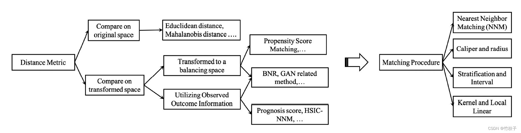
3. matching methods*
4. tree-based methods*
This approach is different from conventional CART in two aspects. First, it focuses on estimating conditional average treatment effects instead of directly predicting outcomes as in the conventional CART. Second, different samples are used for constructing the partition and estimating the effects of each subpopulation, which is referred to as an honest estimation. However, in the conventional CART, the same samples are used for these two tasks.
5. representation based methods
1. Domain Adaptation Based on Representation Learning
Unlike the randomized control trials, the mechanism of treatment assignment is not explicit in observational data. The counterfactual distribution will generally be
different from the factual distribution.
关键在于缩小反事实分布和实际分布的差别,即源域和目标域
6. multi-task methods
7. meta-learning methods*
1. S-learner
S-learner是将treatment作为特征,所有数据一起训练
- step1: μ ( T , X ) = E [ Y ∣ T , X ] \mu(T, X)=E[Y \mid T, X] μ(T,X)=E[Y∣T,X]
- step2: τ ^ = 1 n ∑ i ( μ ^ ( 1 , X i ) − μ ^ ( 0 , X i ) ) \hat{\tau}=\frac{1}{n} \sum_i\left(\hat{\mu}\left(1, X_i\right)-\hat{\mu}\left(0, X_i\right)\right) τ^=n1∑i(μ^(1,Xi)−μ^(0,Xi))
该方法不直接建模uplift,X的high dimension可能会导致treatment丢失效果。
2. T-learner
T-learner分别对control和treatment组建模
- step1: μ 1 ( X ) = E [ Y ∣ T = 1 , X ] μ 0 ( X ) = E [ Y ∣ T = 0 , X ] \mu_1(X)=E[Y \mid T=1, X] \quad \mu_0(X)=E[Y \mid T=0, X] μ1(X)=E[Y∣T=1,X]μ0(X)=E[Y∣T=0,X]
- step2: τ ^ = 1 n ∑ i ( μ ^ 1 ( X i ) − μ 0 ^ ( X i ) ) \hat{\tau}=\frac{1}{n} \sum_i\left(\hat{\mu}_1\left(X_i\right)-\hat{\mu_0}\left(X_i\right)\right) τ^=n1∑i(μ^1(Xi)−μ0^(Xi))
每个estimator只使用部分数据,尤其当样本不足或者treatment、control样本量差别较大时,模型variance较大(对数据利用效率低);容易出现两个模型的Bias方向不一致,形成误差累积,使用时需要针对两个模型打分分布做一定校准;同时当数据差异过大时(如数据量、采样偏差等),对准确率影响较大。
3. X-learner
X-Learner在T-Learner基础上,利用了全量的数据进行预测,主要解决Treatment组间数据量差异较大的情况。
- step1: 对实验组和对照组分别建立两个模型
μ
^
1
\hat \mu_1
μ^1和
μ
^
0
\hat \mu_0
μ^0
D 0 = μ ^ 1 ( X 0 ) − Y 0 D 1 = Y 1 − μ ^ 0 ( X 1 ) \begin{aligned} &D_0=\hat{\mu}_1\left(X_0\right)-Y_0 \\ &D_1=Y_1-\hat{\mu}_0\left(X_1\right) \end{aligned} D0=μ^1(X0)−Y0D1=Y1−μ^0(X1) - step2: 对求得的实验组和对照组增量D1和
D
0
D 0
D0 建立两个模型
τ
^
1
\hat{\tau}_1
τ^1 和
τ
^
0
\hat{\tau}_0
τ^0 。
τ ^ 0 = f ( X 0 , D 0 ) τ ^ 1 = f ( X 1 , D 1 ) \begin{aligned} &\hat{\tau}_0=f\left(X_0, D_0\right) \\ &\hat{\tau}_1=f\left(X_1, D_1\right) \end{aligned} τ^0=f(X0,D0)τ^1=f(X1,D1) - step3: 引入倾向性得分模型
e
(
x
)
e(x)
e(x) 对结果进行加权,求得增量。
e ( x ) = P ( W = 1 ∣ X = x ) τ ^ ( x ) = e ( x ) τ ^ 0 ( x ) + ( 1 − e ( x ) ) τ ^ 1 ( x ) \begin{aligned} &e(x)=P(W=1 \mid X=x) \\ &\hat{\tau}(x)=e(x) \hat{\tau}_0(x)+(1-e(x)) \hat{\tau}_1(x) \end{aligned} e(x)=P(W=1∣X=x)τ^(x)=e(x)τ^0(x)+(1−e(x))τ^1(x)
4. R-learner


 323
323


 被折叠的 条评论
为什么被折叠?
被折叠的 条评论
为什么被折叠?
 到【灌水乐园】发言


