


一直关注公众号的小伙伴想必通过蚁群算法通俗讲解(附MATLAB代码)这篇推文已经了解了蚁群算法(ACO)的基本思想。今天在此基础上,我们分析ACO参数对算法性能的影响。
▎实际案例
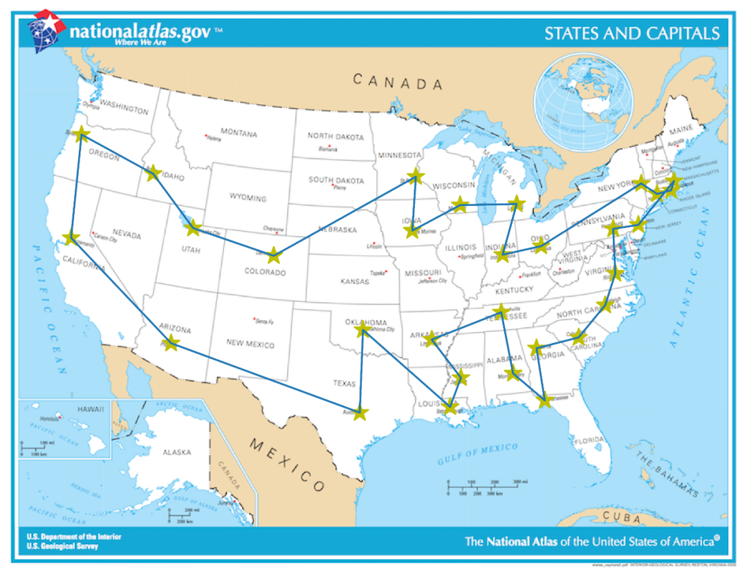
求解下述标星位置的最短路线,具体位置信息如下所示。

cities = { "Oklahoma City": (392.8, 356.4), "Montgomery": (559.6, 404.8),
           "Saint Paul": (451.6, 186.0), "Trenton": (698.8, 239.6),
           "Salt Lake City": (204.0, 243.2), "Columbus": (590.8, 263.2),
           "Austin": (389.2, 448.4), "Phoenix": (179.6, 371.2),
           "Hartford": (719.6, 205.2), "Baton Rouge": (489.6, 442.0),
           "Salem": (80.0, 139.2), "Little Rock": (469.2, 367.2),
           "Richmond": (673.2, 293.6), "Jackson": (501.6, 409.6),
           "Des Moines": (447.6, 246.0), "Lansing": (563.6, 216.4),
           "Denver": (293.6, 274.0), "Boise": (159.6, 182.8),
           "Raleigh": (662.0, 328.8), "Atlanta": (585.6, 376.8),
           "Madison": (500.8, 217.6), "Indianapolis": (548.0, 272.8),
           "Nashville": (546.4, 336.8), "Columbia": (632.4, 364.8),
           "Providence": (735.2, 201.2), "Boston": (738.4, 190.8),
           "Tallahassee": (594.8, 434.8), "Sacramento": (68.4, 254.0),
           "Albany": (702.0, 193.6), "Harrisburg": (670.8, 244.0) }
▎ACO算法求解TSP问题Python代码
ACO算法求解TSP问题Python代码如下:
目录
Data.py读取位置数据,绘制路线图。
import numpy as np
import math
import matplotlib.pyplot as plt
import matplotlib.image as mpimg

united_states_map = mpimg.imread("united_states_map.png")

def show_cities(path, w=12, h=8):
    """Plot a TSP path overlaid on a map of the US States & their capitals."""
    if isinstance(path, dict):      path = list(path.values())
    if isinstance(path[0][0], str): path = [item[1] for item in path]
    plt.imshow(united_states_map)
    for x0, y0 in path:
        plt.plot(x0, y0, 'y*', markersize=15)  # y* = yellow star for starting point
    plt.axis("off")
    fig = plt.gcf()
    fig.set_size_inches([w, h])

def show_path(path, starting_city=None, w=12, h=8):
    """Plot a TSP path overlaid on a map of the US States & their capitals."""
    if isinstance(path, dict):      path = list(path.values())
    if isinstance(path[0][0], str): path = [item[1] for item in path]

    starting_city = starting_city or path[0]
    x, y = list(zip(*path))
    # _, (x0, y0) = starting_city
    (x0, y0) = starting_city
    plt.imshow(united_states_map)
    # plt.plot(x0, y0, 'y*', markersize=15)  # y* = yellow star for starting point
    plt.plot(x + x[:1], y + y[:1])  # include the starting point at the end of path
    plt.axis("off")
    fig = plt.gcf()
    fig.set_size_inches([w, h])

def polyfit_plot(x, y, deg, **kwargs):
    coefficients = np.polyfit(x, y, deg, **kwargs)
    poly = np.poly1d(coefficients)
    new_x = np.linspace(x[0], x[-1])
    new_y = poly(new_x)
    plt.plot(x, y, "o", new_x, new_y)
    plt.xlim([x[0] - 1, x[-1] + 1])

    terms = []
    for p, c in enumerate(reversed(coefficients)):
        term = str(round(c, 1))
        if p == 1: term += 'x'
        if p >= 2: term += 'x^' + str(p)
        terms.append(term)
    plt.title(" + ".join(reversed(terms)))

def distance(xy1, xy2) -> float:
    if isinstance(xy1[0], str): xy1 = xy1[1]; xy2 = xy2[1];               # if xy1 == ("Name", (x,y))
    return math.sqrt( (xy1[0]-xy2[0])**2 + (xy1[1]-xy2[1])**2 )

def path_distance(path) -> int:
    if isinstance(path, dict):      path = list(path.values())            # if path == {"Name": (x,y)}
    if isinstance(path[0][0], str): path = [ item[1] for item in path ]   # if path == ("Name", (x,y))
    return int(sum(
        [ distance(path[i],  path[i+1]) for i in range(len(path)-1) ]
      + [ distance(path[-1], path[0]) ]                                   # include cost of return journey
    ))

cities = { "Oklahoma City": (392.8, 356.4), "Montgomery": (559.6, 404.8),
           "Saint Paul": (451.6, 186.0), "Trenton": (698.8, 239.6),
           "Salt Lake City": (204.0, 243.2), "Columbus": (590.8, 263.2),
           "Austin": (389.2, 448.4), "Phoenix": (179.6, 371.2),
           "Hartford": (719.6, 205.2), "Baton Rouge": (489.6, 442.0),
           "Salem": (80.0, 139.2), "Little Rock": (469.2, 367.2),
           "Richmond": (673.2, 293.6), "Jackson": (501.6, 409.6),
           "Des Moines": (447.6, 246.0), "Lansing": (563.6, 216.4),
           "Denver": (293.6, 274.0), "Boise": (159.6, 182.8),
           "Raleigh": (662.0, 328.8), "Atlanta": (585.6, 376.8),
           "Madison": (500.8, 217.6), "Indianapolis": (548.0, 272.8),
           "Nashville": (546.4, 336.8), "Columbia": (632.4, 364.8),
           "Providence": (735.2, 201.2), "Boston": (738.4, 190.8),
           "Tallahassee": (594.8, 434.8), "Sacramento": (68.4, 254.0),
           "Albany": (702.0, 193.6), "Harrisburg": (670.8, 244.0) }
cities = list(sorted(cities.items()))
print(len(cities))
show_cities(cities)
求解结果如下所示:
{'path_cost': 4118, 'ants_used': 1, 'epoch': 3717, 'round_trips': 1, 'clock': 0}
{'path_cost': 3942, 'ants_used': 86, 'epoch': 9804, 'round_trips': 2, 'clock': 0}
{'path_cost': 3781, 'ants_used': 133, 'epoch': 12887, 'round_trips': 3, 'clock': 0}
{'path_cost': 3437, 'ants_used': 135, 'epoch': 12900, 'round_trips': 3, 'clock': 0}
{'path_cost': 3428, 'ants_used': 138, 'epoch': 13019, 'round_trips': 3, 'clock': 0}
{'path_cost': 3192, 'ants_used': 143, 'epoch': 13339, 'round_trips': 3, 'clock': 0}
{'path_cost': 2981, 'ants_used': 193, 'epoch': 15646, 'round_trips': 4, 'clock': 0}
{'path_cost': 2848, 'ants_used': 198, 'epoch': 15997, 'round_trips': 4, 'clock': 0}
{'path_cost': 2760, 'ants_used': 199, 'epoch': 16030, 'round_trips': 4, 'clock': 0}
{'path_cost': 2757, 'ants_used': 216, 'epoch': 16770, 'round_trips': 4, 'clock': 0}
{'path_cost': 2662, 'ants_used': 222, 'epoch': 16973, 'round_trips': 4, 'clock': 0}
{'path_cost': 2600, 'ants_used': 263, 'epoch': 18674, 'round_trips': 5, 'clock': 0}
{'path_cost': 2504, 'ants_used': 276, 'epoch': 19218, 'round_trips': 5, 'clock': 0}
{'path_cost': 2442, 'ants_used': 284, 'epoch': 19338, 'round_trips': 5, 'clock': 0}
{'path_cost': 2313, 'ants_used': 326, 'epoch': 20982, 'round_trips': 6, 'clock': 0}
{'path_cost': 2226, 'ants_used': 728, 'epoch': 35648, 'round_trips': 12, 'clock': 0}
N=30  |  7074 -> 2240 |    2s | ants:  1727 | trips:   28 | distance_power=1
[('Albany', (702.0, 193.6)), ('Hartford', (719.6, 205.2)), ('Providence', (735.2, 201.2)), ('Boston', (738.4, 190.8)), ('Trenton', (698.8, 239.6)), ('Harrisburg', (670.8, 244.0)), ('Richmond', (673.2, 293.6)), ('Raleigh', (662.0, 328.8)), ('Columbia', (632.4, 364.8)), ('Atlanta', (585.6, 376.8)), ('Montgomery', (559.6, 404.8)), ('Tallahassee', (594.8, 434.8)), ('Baton Rouge', (489.6, 442.0)), ('Jackson', (501.6, 409.6)), ('Little Rock', (469.2, 367.2)), ('Oklahoma City', (392.8, 356.4)), ('Austin', (389.2, 448.4)), ('Phoenix', (179.6, 371.2)), ('Sacramento', (68.4, 254.0)), ('Salem', (80.0, 139.2)), ('Boise', (159.6, 182.8)), ('Salt Lake City', (204.0, 243.2)), ('Denver', (293.6, 274.0)), ('Des Moines', (447.6, 246.0)), ('Saint Paul', (451.6, 186.0)), ('Madison', (500.8, 217.6)), ('Lansing', (563.6, 216.4)), ('Columbus', (590.8, 263.2)), ('Indianapolis', (548.0, 272.8)), ('Nashville', (546.4, 336.8)), ('Nashville', (546.4, 336.8)), ('Albany', (702.0, 193.6))]▎ACO算法性能分析
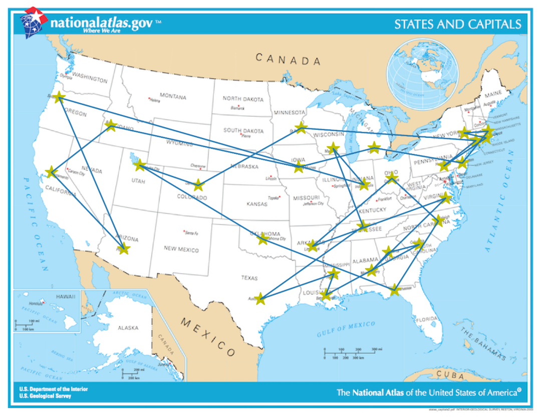
01 | 当不考虑启发因子,仅考虑信息素时
results = AntColonyRunner(cities, distance_power=0, min_time=30, verbose=True, plot=True)
求解结果如下:
{'path_cost': 6700, 'ants_used': 1, 'epoch': 6202, 'round_trips': 1, 'clock': 0}
{'path_cost': 6693, 'ants_used': 2, 'epoch': 6522, 'round_trips': 1, 'clock': 0}
{'path_cost': 5986, 'ants_used': 67, 'epoch': 13559, 'round_trips': 2, 'clock': 0}
{'path_cost': 5902, 'ants_used': 391, 'epoch': 50120, 'round_trips': 7, 'clock': 0}
{'path_cost': 5886, 'ants_used': 473, 'epoch': 59009, 'round_trips': 8, 'clock': 0}
{'path_cost': 5683, 'ants_used': 514, 'epoch': 62612, 'round_trips': 9, 'clock': 0}
{'path_cost': 5516, 'ants_used': 591, 'epoch': 72020, 'round_trips': 10, 'clock': 0}
{'path_cost': 5297, 'ants_used': 648, 'epoch': 77733, 'round_trips': 11, 'clock': 1}
{'path_cost': 5290, 'ants_used': 671, 'epoch': 79463, 'round_trips': 11, 'clock': 1}
{'path_cost': 5192, 'ants_used': 684, 'epoch': 80368, 'round_trips': 11, 'clock': 1}
{'path_cost': 4359, 'ants_used': 707, 'epoch': 83222, 'round_trips': 12, 'clock': 1}
N=30  |  7074 -> 4375 |    1s | ants:   958 | trips:   16 | distance_power=0 stop_factor=1.25
实验结果表明,仅考虑信息素,而不考虑启发因子,求解质量严重下降。
02 | 启发因子距离权重
启发因子距离权重n影响蚂蚁在选择下一节点时“看见”距离的能力,而不仅仅盲目地依赖信息素。接下来将距离权重n取不同值进行实验,验证其对求解质量的影响。
for distance_power in [-2.0, -1.0, 0.0, 0.5, 1.0, 1.25, 1.5, 1.75, 2.0, 3.0, 5.0, 10.0]:
    result = AntColonyRunner(cities, distance_power=distance_power, timeout=60)
求解结果如下:
N=30  |  7074 -> 8225 |    1s | ants:   577 | trips:   10 | distance_power=-2.0 timeout=60
N=30  |  7074 -> 7957 |    1s | ants:   577 | trips:   10 | distance_power=-1.0 timeout=60
N=30  |  7074 -> 3947 |   22s | ants: 12439 | trips:  196 | distance_power=0.0 timeout=60
N=30  |  7074 -> 2558 |    7s | ants:  4492 | trips:   72 | distance_power=0.5 timeout=60
N=30  |  7074 -> 2227 |    2s | ants:  1168 | trips:   19 | distance_power=1.0 timeout=60
N=30  |  7074 -> 2290 |    4s | ants:  2422 | trips:   39 | distance_power=1.25 timeout=60
N=30  |  7074 -> 2367 |    1s | ants:   679 | trips:   11 | distance_power=1.5 timeout=60
N=30  |  7074 -> 2211 |    2s | ants:  1412 | trips:   23 | distance_power=1.75 timeout=60
N=30  |  7074 -> 2298 |    7s | ants:  4429 | trips:   70 | distance_power=2.0 timeout=60
N=30  |  7074 -> 2200 |    2s | ants:  1411 | trips:   23 | distance_power=3.0 timeout=60
N=30  |  7074 -> 2232 |    1s | ants:   758 | trips:   12 | distance_power=5.0 timeout=60
N=30  |  7074 -> 2240 |    1s | ants:   577 | trips:   10 | distance_power=10.0 timeout=60
实验结果表明:
1.当n取负数时,鼓励蚂蚁先到更远的节点,因此出现求解结果比随机路线更差的情况。
2.当n=0时,蚂蚁完全依赖信息素选择下一节点。
3.当n=1时,求解质量较好,但是在间隔紧密的节点周围存在一些“循环”路线。
4.当n=1.25~2时,算法收敛更快,求解质量更佳(通常默认n=2)。
5.当n大于等于3时,算法收敛速度过快,导致算法搜索空间缩小,求解质量下降。
03 | 信息素权重
信息素权重影响信息素的相对差异被注意到的能力。接下来将信息素权重取不同值进行实验,验证其对求解质量的影响。
第1轮实验:
for distance_power in [0,1,2]:
    for pheromone_power in [-2.0, -1.0, 0.0, 0.5, 1.0, 1.25, 1.5, 1.75, 2.0, 3.0, 5.0, 10.0]:
        result = AntColonyRunner(cities, distance_power=distance_power, pheromone_power=pheromone_power, time=0)
    print()
第1轮实验求解结果如下:
N=30  |  7074 -> 5477 |    1s | ants:   574 | trips:   10 | distance_power=0 pheromone_power=-2.0 time=0
N=30  |  7074 -> 5701 |    1s | ants:   688 | trips:   11 | distance_power=0 pheromone_power=-1.0 time=0
N=30  |  7074 -> 6039 |    2s | ants:   570 | trips:   10 | distance_power=0 pheromone_power=0.0 time=0
N=30  |  7074 -> 5970 |    2s | ants:   689 | trips:   11 | distance_power=0 pheromone_power=0.5 time=0
N=30  |  7074 -> 5628 |    2s | ants:   573 | trips:   10 | distance_power=0 pheromone_power=1.0 time=0
N=30  |  7074 -> 5246 |    2s | ants:   894 | trips:   15 | distance_power=0 pheromone_power=1.25 time=0
N=30  |  7074 -> 4035 |   13s | ants:  7217 | trips:  114 | distance_power=0 pheromone_power=1.5 time=0
N=30  |  7074 -> 4197 |    9s | ants:  4602 | trips:   73 | distance_power=0 pheromone_power=1.75 time=0
N=30  |  7074 -> 4328 |    3s | ants:  1788 | trips:   29 | distance_power=0 pheromone_power=2.0 time=0
N=30  |  7074 -> 4188 |    1s | ants:   700 | trips:   11 | distance_power=0 pheromone_power=3.0 time=0
N=30  |  7074 -> 5151 |    1s | ants:   577 | trips:   10 | distance_power=0 pheromone_power=5.0 time=0
N=30  |  7074 -> 5278 |    1s | ants:   577 | trips:   10 | distance_power=0 pheromone_power=10.0 time=0

N=30  |  7074 -> 4444 |    1s | ants:   561 | trips:   10 | distance_power=1 pheromone_power=-2.0 time=0
N=30  |  7074 -> 4035 |    1s | ants:   564 | trips:   10 | distance_power=1 pheromone_power=-1.0 time=0
N=30  |  7074 -> 4016 |    1s | ants:   788 | trips:   13 | distance_power=1 pheromone_power=0.0 time=0
N=30  |  7074 -> 2733 |    4s | ants:  1968 | trips:   32 | distance_power=1 pheromone_power=0.5 time=0
N=30  |  7074 -> 2263 |    3s | ants:  2424 | trips:   39 | distance_power=1 pheromone_power=1.0 time=0
N=30  |  7074 -> 2315 |    2s | ants:  1863 | trips:   30 | distance_power=1 pheromone_power=1.25 time=0
N=30  |  7074 -> 2528 |    1s | ants:  1107 | trips:   18 | distance_power=1 pheromone_power=1.5 time=0
N=30  |  7074 -> 2593 |    1s | ants:   615 | trips:   10 | distance_power=1 pheromone_power=1.75 time=0
N=30  |  7074 -> 2350 |    1s | ants:   631 | trips:   10 | distance_power=1 pheromone_power=2.0 time=0
N=30  |  7074 -> 2806 |    1s | ants:   680 | trips:   11 | distance_power=1 pheromone_power=3.0 time=0
N=30  |  7074 -> 3079 |    1s | ants:   577 | trips:   10 | distance_power=1 pheromone_power=5.0 time=0
N=30  |  7074 -> 3087 |    1s | ants:   577 | trips:   10 | distance_power=1 pheromone_power=10.0 time=0

N=30  |  7074 -> 3277 |    1s | ants:   558 | trips:   10 | distance_power=2 pheromone_power=-2.0 time=0
N=30  |  7074 -> 3191 |    1s | ants:   536 | trips:   10 | distance_power=2 pheromone_power=-1.0 time=0
N=30  |  7074 -> 2958 |    2s | ants:  1124 | trips:   19 | distance_power=2 pheromone_power=0.0 time=0
N=30  |  7074 -> 2229 |    4s | ants:  3027 | trips:   49 | distance_power=2 pheromone_power=0.5 time=0
N=30  |  7074 -> 2432 |    1s | ants:   560 | trips:   10 | distance_power=2 pheromone_power=1.0 time=0
N=30  |  7074 -> 2275 |    5s | ants:  4391 | trips:   70 | distance_power=2 pheromone_power=1.25 time=0
N=30  |  7074 -> 2320 |    3s | ants:  2194 | trips:   35 | distance_power=2 pheromone_power=1.5 time=0
N=30  |  7074 -> 2534 |    1s | ants:   778 | trips:   13 | distance_power=2 pheromone_power=1.75 time=0
N=30  |  7074 -> 2233 |    1s | ants:   938 | trips:   15 | distance_power=2 pheromone_power=2.0 time=0
N=30  |  7074 -> 2308 |    1s | ants:   897 | trips:   15 | distance_power=2 pheromone_power=3.0 time=0
N=30  |  7074 -> 2320 |    1s | ants:   645 | trips:   11 | distance_power=2 pheromone_power=5.0 time=0
N=30  |  7074 -> 2653 |    1s | ants:   577 | trips:   10 | distance_power=2 pheromone_power=10.0 time=0
第2轮实验:
for distance_power in [0,1,2]:
    for pheromone_power in [-2.0, -1.0, 0.0, 0.5, 1.0, 1.25, 1.5, 1.75, 2.0, 3.0, 5.0, 10.0]:
        result = AntColonyRunner(cities, distance_power=distance_power, pheromone_power=pheromone_power, time=0)
    print()
第2轮实验求解结果如下:
N=30  |  7074 -> 5842 |    2s | ants:   577 | trips:   10 | distance_power=0 pheromone_power=-2.0 time=0
N=30  |  7074 -> 5897 |    3s | ants:  1080 | trips:   18 | distance_power=0 pheromone_power=-1.0 time=0
N=30  |  7074 -> 5798 |    1s | ants:   574 | trips:   10 | distance_power=0 pheromone_power=0.0 time=0
N=30  |  7074 -> 6059 |    1s | ants:   570 | trips:   10 | distance_power=0 pheromone_power=0.5 time=0
N=30  |  7074 -> 4068 |    7s | ants:  3562 | trips:   57 | distance_power=0 pheromone_power=1.0 time=0
N=30  |  7074 -> 3620 |    3s | ants:  2553 | trips:   41 | distance_power=0 pheromone_power=1.25 time=0
N=30  |  7074 -> 3994 |    5s | ants:  2822 | trips:   45 | distance_power=0 pheromone_power=1.5 time=0
N=30  |  7074 -> 4067 |    3s | ants:  2210 | trips:   35 | distance_power=0 pheromone_power=1.75 time=0
N=30  |  7074 -> 4232 |    3s | ants:  2057 | trips:   33 | distance_power=0 pheromone_power=2.0 time=0
N=30  |  7074 -> 4559 |    2s | ants:  1179 | trips:   19 | distance_power=0 pheromone_power=3.0 time=0
N=30  |  7074 -> 4566 |    1s | ants:   575 | trips:   10 | distance_power=0 pheromone_power=5.0 time=0
N=30  |  7074 -> 5565 |    1s | ants:   577 | trips:   10 | distance_power=0 pheromone_power=10.0 time=0

N=30  |  7074 -> 4377 |    1s | ants:   570 | trips:   10 | distance_power=1 pheromone_power=-2.0 time=0
N=30  |  7074 -> 4459 |    1s | ants:   535 | trips:   10 | distance_power=1 pheromone_power=-1.0 time=0
N=30  |  7074 -> 4269 |    1s | ants:   559 | trips:   10 | distance_power=1 pheromone_power=0.0 time=0
N=30  |  7074 -> 3144 |    1s | ants:   636 | trips:   11 | distance_power=1 pheromone_power=0.5 time=0
N=30  |  7074 -> 2371 |    2s | ants:  1265 | trips:   21 | distance_power=1 pheromone_power=1.0 time=0
N=30  |  7074 -> 2298 |    4s | ants:  2880 | trips:   47 | distance_power=1 pheromone_power=1.25 time=0
N=30  |  7074 -> 2337 |    7s | ants:  4058 | trips:   65 | distance_power=1 pheromone_power=1.5 time=0
N=30  |  7074 -> 2317 |    2s | ants:  1647 | trips:   27 | distance_power=1 pheromone_power=1.75 time=0
N=30  |  7074 -> 2386 |    2s | ants:   808 | trips:   13 | distance_power=1 pheromone_power=2.0 time=0
N=30  |  7074 -> 2434 |    1s | ants:   573 | trips:   10 | distance_power=1 pheromone_power=3.0 time=0
N=30  |  7074 -> 2776 |    1s | ants:   578 | trips:   10 | distance_power=1 pheromone_power=5.0 time=0
N=30  |  7074 -> 3255 |    1s | ants:   577 | trips:   10 | distance_power=1 pheromone_power=10.0 time=0

N=30  |  7074 -> 2748 |    1s | ants:   560 | trips:   10 | distance_power=2 pheromone_power=-2.0 time=0
N=30  |  7074 -> 3224 |    1s | ants:   542 | trips:   10 | distance_power=2 pheromone_power=-1.0 time=0
N=30  |  7074 -> 2958 |    1s | ants:   543 | trips:   10 | distance_power=2 pheromone_power=0.0 time=0
N=30  |  7074 -> 2705 |    2s | ants:   816 | trips:   14 | distance_power=2 pheromone_power=0.5 time=0
N=30  |  7074 -> 2205 |    2s | ants:  1033 | trips:   17 | distance_power=2 pheromone_power=1.0 time=0
N=30  |  7074 -> 2301 |    2s | ants:  1071 | trips:   17 | distance_power=2 pheromone_power=1.25 time=0
N=30  |  7074 -> 2248 |    2s | ants:  1171 | trips:   19 | distance_power=2 pheromone_power=1.5 time=0
N=30  |  7074 -> 2194 |    2s | ants:  1001 | trips:   16 | distance_power=2 pheromone_power=1.75 time=0
N=30  |  7074 -> 2371 |    1s | ants:   575 | trips:   10 | distance_power=2 pheromone_power=2.0 time=0
N=30  |  7074 -> 2338 |    2s | ants:  1310 | trips:   21 | distance_power=2 pheromone_power=3.0 time=0
N=30  |  7074 -> 2371 |    1s | ants:   576 | trips:   10 | distance_power=2 pheromone_power=5.0 time=0
N=30  |  7074 -> 2942 |    1s | ants:   577 | trips:   10 | distance_power=2 pheromone_power=10.0 time=0
第3轮实验:
for distance_power in [0,1,2]:
    for pheromone_power in [1.0, 1.1, 1.2, 1.3, 1.4]:
        result = AntColonyRunner(cities, distance_power=distance_power, pheromone_power=pheromone_power, time=0)
    print()
第3轮实验求解结果如下:
N=30  |  7074 -> 5107 |    1s | ants:   764 | trips:   13 | distance_power=0 pheromone_power=1.0 time=0
N=30  |  7074 -> 3393 |   15s | ants:  8420 | trips:  134 | distance_power=0 pheromone_power=1.1 time=0
N=30  |  7074 -> 3548 |   20s | ants: 12669 | trips:  200 | distance_power=0 pheromone_power=1.2 time=0
N=30  |  7074 -> 4267 |    2s | ants:   831 | trips:   14 | distance_power=0 pheromone_power=1.3 time=0
N=30  |  7074 -> 5194 |    1s | ants:   562 | trips:   10 | distance_power=0 pheromone_power=1.4 time=0

N=30  |  7074 -> 2231 |    3s | ants:  1507 | trips:   25 | distance_power=1 pheromone_power=1.0 time=0
N=30  |  7074 -> 2297 |    4s | ants:  2213 | trips:   36 | distance_power=1 pheromone_power=1.1 time=0
N=30  |  7074 -> 2399 |    5s | ants:  2586 | trips:   41 | distance_power=1 pheromone_power=1.2 time=0
N=30  |  7074 -> 2274 |    3s | ants:  1365 | trips:   22 | distance_power=1 pheromone_power=1.3 time=0
N=30  |  7074 -> 2323 |    2s | ants:  1164 | trips:   19 | distance_power=1 pheromone_power=1.4 time=0

N=30  |  7074 -> 2244 |    3s | ants:  1724 | trips:   28 | distance_power=2 pheromone_power=1.0 time=0
N=30  |  7074 -> 2240 |    3s | ants:  1518 | trips:   25 | distance_power=2 pheromone_power=1.1 time=0
N=30  |  7074 -> 2251 |    3s | ants:  1736 | trips:   28 | distance_power=2 pheromone_power=1.2 time=0
N=30  |  7074 -> 2259 |    1s | ants:   895 | trips:   15 | distance_power=2 pheromone_power=1.3 time=0
N=30  |  7074 -> 2257 |    6s | ants:  4397 | trips:   70 | distance_power=2 pheromone_power=1.4 time=0
实验结果表面:
1.负数使信息素被排斥,但是求解结果仍比随机结果更优。
2.蚂蚁对信息大于1的信息素较为敏感,稍微增加一点就会大幅度改进求解结果,但会增加算法求解时间。
3.通常默认信息素权重取值1.25。
04 | 蚂蚁数量
我们的直觉是蚂蚁数量越大,收敛速度更快,求解质量更好,那么结果究竟是否如此,下面的实验为我们揭晓答案。
for ant_count in range(0,16+1):
    AntColonyRunner(cities, ant_count=2**ant_count, time=60)
求解结果如下:
N=30  |  7074 -> 2711 |   60s | ants:  3722 | trips: 3722 | ant_count=1 time=60
N=30  |  7074 -> 2785 |   60s | ants:  6094 | trips: 3047 | ant_count=2 time=60
N=30  |  7074 -> 2228 |   60s | ants: 14719 | trips: 3682 | ant_count=4 time=60
N=30  |  7074 -> 2338 |   60s | ants: 23195 | trips: 2902 | ant_count=8 time=60
N=30  |  7074 -> 2465 |   60s | ants: 27378 | trips: 1714 | ant_count=16 time=60
N=30  |  7074 -> 2430 |   60s | ants: 41132 | trips: 1291 | ant_count=32 time=60
N=30  |  7074 -> 2262 |   60s | ants: 43098 | trips:  676 | ant_count=64 time=60
N=30  |  7074 -> 2210 |   60s | ants: 63140 | trips:  496 | ant_count=128 time=60
N=30  |  7074 -> 2171 |   60s | ants: 68796 | trips:  272 | ant_count=256 time=60
N=30  |  7074 -> 2196 |   60s | ants: 67791 | trips:  134 | ant_count=512 time=60
N=30  |  7074 -> 2203 |   60s | ants: 73140 | trips:   73 | ant_count=1024 time=60
N=30  |  7074 -> 2227 |   60s | ants: 81049 | trips:   41 | ant_count=2048 time=60
N=30  |  7074 -> 2196 |   60s | ants: 73486 | trips:   19 | ant_count=4096 time=60
N=30  |  7074 -> 2210 |   60s | ants: 71547 | trips:   10 | ant_count=8192 time=60
N=30  |  7074 -> 2176 |   60s | ants: 63254 | trips:    5 | ant_count=16384 time=60
N=30  |  7074 -> 2357 |   60s | ants: 33481 | trips:    2 | ant_count=32768 time=60
N=30  |  7074 -> 3490 |   61s | ants: 10391 | trips:    1 | ant_count=65536 time=60
实验结果表明:
1.蚂蚁数量在64~16384之间,ACO求解质量较佳。
2.当蚂蚁数量大于32768时,ACO求解质量急剧下降。
▎总结
我们通过这期推文分析了距离权重、信息素权重和蚂蚁数量对ACO性能的影响,初步结论为距离权重通常设为2,信息素权重通常设为1.25,蚂蚁数量取值范围为64~16384。
▎参考
[1]https://www.kaggle.com/code/jamesmcguigan/ant-colony-optimization-algorithm/notebook
咱们下期再见
▎近期你可能错过了的好文章
新书上架 | 《MATLAB智能优化算法:从写代码到算法思想》


 6874
6874


 被折叠的 条评论
为什么被折叠?
被折叠的 条评论
为什么被折叠?
 到【灌水乐园】发言


