优化算法 | 单纯形法（附MATLAB代码）

hello，大家好。各位可点击左下方阅读原文，访问公众号官方店铺。谨防上当受骗，感谢各位支持！如果链接无法访问，公众号后台回复代码商店，即可获取官方店铺最新链接。

Hello，各位小伙伴。前一段时间二刷了方述诚老师的《线性规划》公开课，不由得再次感叹方老师讲得实在是太好了。

《线性规划》公开课视频链接为：https://b23.tv/h1uTSbZ

今天这期推文作为年前收官之作，主要是谈一下对单纯形法的理解。

我想绝大多数同学之前在学校上最优化或运筹学课程时，老师几乎都是教我们用单纯形表来求解一个问题，然后我们也就机械地按步骤去操作做题。但实际上，无论是单纯形法还是智能优化算法，我认为它们的内核都是一致的，那就是通过迭代更新位置的方式去搜索更优质的解。

因此，在《线性规划》这门课中，方老师讲到了单纯形法的初始解构造方法、位置更新公式和最优解判别标准。

因为在单纯形法中，找到一个初始解和从一个可行解找到最优解的难度几乎相同，所以在后续小节中，我们按照位置更新公式、最优解判别标准和初始解构造方法来讲解。

---

预备知识

线性规划（LP）标准形式

$$\begin{array}{r}\mathrm{Min}{\mathbf{c}}^T\mathbf{x}\\ \text{ s.t. }\mathbf{Ax}=\mathbf{b}\\ \mathbf{x}\ge 0\end{array}$$

其中，cost vector $\mathbf{c}={\left(c_1,c_2,\cdots ,c_n\right)}^T$，solution vector $\mathbf{x}={\left(x_1,x_2,\cdots ,x_n\right)}^T$，right-hand-side vector $\mathbf{b}={\left(b_1,b_2,\cdots ,b_n\right)}^T$，

constraint matrix $\mathbf{A}=\left(\begin{array}{cccc}{a}_{11}& a_{12}& \cdots & a_{1n}\\ a_{21}& a_{22}& \cdots & a_{2n}\\ ⋮& ⋮& \ddots & ⋮\\ a_{m1}& a_{m2}& \cdots & a_{mn}\end{array}\right)$。

超平面（hyperplane）

标准形式LP中的每一项等式约束都视为解空间中的一个超平面。

【超平面定义】对于一个向量$\mathbf{a}\in {\mathbf{R}}^n,\mathbf{a}\ne 0$，和一个实数$\beta \in \mathbf{R}$，超平面$H=\left\{\mathrm{x}\in {\mathbf{R}}^n\mid {\mathrm{a}}^T\mathrm{x}=\beta \right\}$。

其中$H_U=\left\{x\text{ in }{R}^n\mid a^{T}x\ge \beta \right\}$和$H_L=\left\{x\text{ in }{R}^n\mid a^{T}x\le \beta \right\}$分别表示上、下半封闭空间，$H_U^i=H_U-H=\left\{x\text{ in }{R}^n\mid a^{T}x>\beta \right\}$和$H_L^i=H_L-H=\left\{x\text{ in }{R}^n\mid a^{T}x<\beta \right\}$分别表示上、下半开放空间。

【性质1】正交向量$a$垂直于超平面$H$中的所有向量。

【性质2】正交向量指向上半个超平面，即指向目标函数值增加的方向。

多面体集合（polyhedral set）

一个多面体集合由有限个半封闭空间相交而成。

【性质3】标准形式LP的可行域 P = { x ∈ R n ∣ A x = b , x ≥ 0 } P=\left\{\mathrm{x} \in \mathrm{R}^n \mid \mathrm{Ax}=\mathrm{b}, \mathrm{x} \geq 0\right\} P={x∈Rn∣Ax=b,x≥0}为一个多面体集合。

线性/仿射/锥/凸组合

【线性组合定义】假设${\mathbf{x}}^1,{\mathbf{x}}^2,\dots ,{\mathbf{x}}^p\in {\mathbf{R}}^n$，${\lambda }_1,{\lambda }_2,\dots ,{\lambda }_p\in \mathbf{R}$和$\mathbf{x}={\sum }_{i=1}^p{\lambda }_i{\mathrm{x}}^i={\lambda }_1{\mathrm{x}}^1+{\lambda }_2{\mathrm{x}}^2+\cdots +{\lambda }_p{\mathrm{x}}^p$，则称$x$是$\left\{{\mathrm{x}}^1,\dots ,{\mathrm{x}}^p\right\}$的线性组合。

【仿射组合定义】基于线性组合假设前提，另如果${\sum }_{i=1}^p{\lambda }_i=1$，则称$x$是$\left\{{\mathrm{x}}^1,\dots ,{\mathrm{x}}^p\right\}$的仿射组合。

【锥组合定义】基于线性组合假设前提，另如果${\lambda }_i\ge 0$，则称$x$是$\left\{{\mathrm{x}}^1,\dots ,{\mathrm{x}}^p\right\}$的锥组合。

【凸组合定义】基于线性组合假设前提，另如果${\sum }_{i=1}^p{\lambda }_i=1,{\lambda }_i\ge 0$，则称$x$是$\left\{{\mathrm{x}}^1,\dots ,{\mathrm{x}}^p\right\}$的凸组合。

仿射集合/凸集合/锥

【仿射集合定义】假设$S$是实数集${\mathbf{R}}^n$的子集，如果$S$中任意两点的仿射组合仍在$S$中，则称$S$为仿射集合。

【凸集合】假设$S$是实数集${\mathbf{R}}^n$的子集，如果$S$中任意两点的凸组合仍在$S$中，则称$S$为凸集合。

【锥】假设$S$是实数集${\mathbf{R}}^n$的子集，如果$\lambda \mathrm{x}\in S\text{ for all }\mathrm{x}\in S\text{ and }\lambda \ge 0$，则称$S$为锥。

极点（extreme point，ep）

【极点定义】如果$x$不能被凸集合$S$内的其它点表示为凸组合的形式，那么$x$是凸集合$S$中的一个极点。

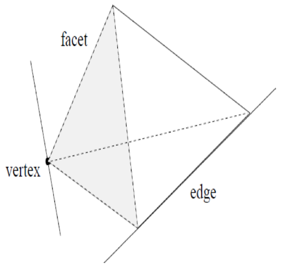
【定理1】假设$P$是一个凸多面体，当且仅当$x$是$P$的一个极点时，那么$x\in P$也是一个顶点。

【定理2】当且仅当矩阵$A$对应于$x$为正数的列向量线性无关时， x ∈ P = { x ∈ R n ∣ A x = b , x ≥ 0 } \mathbf{x} \in P=\left\{\mathbf{x} \in \mathbf{R}^n \mid \mathbf{A} \mathbf{x}=b, \mathbf{x} \geq 0\right\} x∈P={x∈Rn∣Ax=b,x≥0}为$P$的一个极点。

【定理3】对于一个标准形式LP，如果可行域$P$非空，则在$P$上的最优值$\mathbf{z}={\mathbf{c}}^T\mathbf{x}$或者无下界，或者至少在$P$上的一个极点取到。

基/非基/基变量/非基变量/基解/基可行解

假设$A$为$m$行$n$列的矩阵，并且$A$存在$m$个线性无关的列，则$A$称为满秩矩阵。基于此，将矩阵$A$和解向量$x$进行重写，即将$A$中$m$个线性无关的列放在前$m$列，剩余$n-m$列放在这$m$列之后，则$x$中元素也按照此顺序进行调整。
$$\mathrm{x}=\left(\begin{array}{l}{\mathrm{x}}_B\\ {\mathrm{x}}_N\end{array}\right)\leftarrow \begin{array}{c}\text{basic variables}\\ \text{non-basic variables}\end{array}$$

$$\mathbf{A}=\left(\begin{array}{cc}\mathbf{B}& \mathbf{N}\\ \uparrow & \uparrow \\ \text{ basis }& \text{non-basis}\end{array}\right)$$

因此，$B$为基，$N$为非基，${\mathrm{x}}_B$为基变量（basic variable, bv），${\mathrm{x}}_N$为非基变量（non-basic variable, nbv）。

如果设${\mathrm{x}}_N=0$，对于$\mathrm{Ax}={\mathrm{Bx}}_B=\mathrm{b}$求解出${\mathrm{x}}_B$，则$x$为基解（basic solution，bs）。进一步来说，如果${\mathrm{x}}_B>0$，则$x$为基可行解（basic feasible solution，bfs）。

【引理1】当且仅当$x$是对应于基$B$的基可行解bfs，则$P$中的一个点$x$是$P$中的一个极点。

【引理2】多面体集合$P$包含有限个极点。

基础矩阵（fundamental matrix）

如果一个bfs $x$是一个非退化解，那么$x$由$n$个超平面所唯一确定。

记$\mathbf{A}=[\mathbf{B}\mid \mathbf{N}]$，$\mathbf{x}=\left[\begin{array}{l}{\mathbf{x}}_B\\ {\mathbf{x}}_N\end{array}\right]=\left[\begin{array}{c}{\mathbf{B}}^{-1}\mathbf{b}\\ 0\end{array}\right]$，令$M=\left[\begin{array}{cc}\mathrm{B}& \mathrm{N}\\ 0& \mathrm{I}\end{array}\right]$，则$M$是非奇异矩阵，且$\mathrm{Mx}=\left[\begin{array}{cc}\mathrm{B}& \mathrm{N}\\ 0& \mathrm{I}\end{array}\right]\left[\begin{array}{l}{\mathrm{x}}_B\\ {\mathrm{x}}_N\end{array}\right]=\left[\begin{array}{l}\mathrm{b}\\ 0\end{array}\right]$。因此，$\mathbf{x}=\left[\begin{array}{l}{\mathbf{x}}_B\\ {\mathbf{x}}_N\end{array}\right]={\mathbf{M}}^{-1}\left[\begin{array}{l}\mathrm{b}\\ 0\end{array}\right]$由$n$个线性无关超平面所唯一确定。
$${\mathbf{M}}^{-1}=\left[\begin{array}{cc}{\mathrm{B}}^{-1}& -{\mathrm{B}}^{-1}\mathbf{N}\\ 0& \mathbf{I}\end{array}\right]$$
当${\mathrm{B}}^{-1}$已知时，则${\mathbf{M}}^{-1}$已知。

综上，称${\mathbf{M}}^{-1}$或$\mathbf{M}$为LP的基础矩阵。

---

单纯形法整体框架

本次推文所阐述的单纯形法应用场景是非退化情形，针对退化场景的单纯形法可在方老师的课程中学习。

由【引理1】可知，在非退化情形下，一般来说一个极点对应一个bfs。但是在退化情形下，一个极点可能对应多个bfs。

※bfs表示基可行解※

Phase I:
Step 1: (Starting)
Find an initial basic feasible solution (bfs), or declare P is null.
Phase II:
Step 2: (Checking optimality)
If the current bfs is optimal, STOP!
Step 3: (Pivoting)
Move to a better bfs.
Return to Step 2.

---

位置更新公式

由预备知识中的【定理3】可以得知，标准形式LP问题的最优解一定在可行域的某个极点，也就是凸多面体的顶点。所以求解标准形式的LP问题，可以转化为找出“最好的”那个极点。

假设LP问题的可行域是一个凸多面体集合，那么单纯形法的思想就是沿着凸多面体的边从一个顶点移动到另一个顶点，也可以说从一个bfs/ep更新至另一个相邻的bfs/ep（针对非退化情形），进而找到最优解。

那么从一个bfs更新至另一个bfs的公式实际上和其它优化算法的位置更新公式思想一致，即方向${\mathbf{d}}_q$和步长$\alpha$。
$$\mathbf{x}\leftarrow \mathbf{x}+\alpha {\mathbf{d}}_q$$

方向${\mathbf{d}}_q$

既然要从一个bfs/ep更新至另一个相邻的bfs/ep，那么首先需要明确bfs相邻的定义，其次需要明确如何从众多个相邻的bfs中选择下一个bfs作为更新后的位置。

【bfs相邻定义】如果两个bfs有$m-1$个相同的基变量（指的是变量，而不是数值），那么这两个bfs就是相邻的。

在非退化情形下，每个bfs/ep恰好有$n-m$个相邻的邻居。针对一个bfs，其每一个相邻的bfs都可以通过将一个nbv从0增加到正数（即入基），同时将一个bv从正数减小到0（即出基）的方式到达该bfs。

在了解一个bfs有$n-m$个相邻的邻居后，接下来，我们需要明确该朝哪个方向走前往下一个更好的bfs？

这时候，我们可以用到前面所讲的fundamental matrix，${\mathbf{M}}^{-1}=\left[\begin{array}{cc}{\mathrm{B}}^{-1}& -{\mathrm{B}}^{-1}\mathbf{N}\\ 0& \mathbf{I}\end{array}\right]$，这个矩阵中后$n-m$列$\left[\begin{array}{c}-{\mathbf{B}}^{-1}\mathbf{N}\\ \mathbf{I}\end{array}\right]$实际上就表示可能的$n-m$个方向。

$d_q$是${\mathbf{M}}^{-1}$中对应非基变量$x_q$的列，即为一个可能的移动方向，${\mathrm{d}}_q=\left(\begin{array}{c}-{\mathbf{B}}^{-1}{\mathbf{A}}_q\\ 0\\ ⋮\\ 0\\ 1\\ 0\\ ⋮\\ 0\end{array}\right)$，其中$\mathbf{A}=\left({\mathbf{A}}_1\left|{\mathbf{A}}_2\right|\cdots \mid {\mathbf{A}}_n\right)$。

这里的$d_q$表示一个可能的移动方向，但是我们并不知道该方向是否可行？

这里我们直接给出结论，在非退化情形下，每一个$d_q$都是可行方向。但是在退化情形下，可能存在$d_q$不是可行方向的情况。

既然每一个$d_q$都是可行方向，那么究竟哪个$d_q$是好方向呢？

我们可以通过目标函数值进行判断，具体计算公式如下，其中$\mathbf{z}(\mathbf{x}(\lambda ))$表示新bfs的目标函数值，$\mathbf{z}(\mathbf{x})$表示原bfs的目标函数值。
$$\begin{array}{rl}\mathbf{z}(\mathbf{x}(\lambda ))& ={\mathbf{c}}^T\mathbf{x}(\lambda )\\ & ={\mathbf{c}}^T\left(\mathbf{x}+\lambda {\mathbf{d}}_q\right)\\ & =\mathbf{z}(\mathbf{x})+\lambda \left[{\mathbf{c}}_B^T\mid {\mathbf{c}}_N^T\right]\left(\frac{-{\mathbf{B}}^{-1}{\mathbf{A}}_q}{e_q}\right)\\ & =\mathbf{z}(\mathbf{x})+\lambda \left[c_q-{\mathbf{c}}_B^T{\mathbf{B}}^{-1}{\mathbf{A}}_q\right]\\ & =\mathbf{z}(\mathbf{x})+\lambda r_q\end{array}$$
可以看出，$r_q={\mathrm{c}}^T{\mathrm{d}}_q=c_q-{\mathbf{c}}_B^T{B}^{-1}{\mathrm{A}}_q<0$，即表示目标函数值可以继续减小，那么$d_q$就是一个好方向。

【reduced cost定义】$r_q={\mathrm{c}}^T{\mathrm{d}}_q=c_q-{\mathbf{c}}_B^T{B}^{-1}{\mathrm{A}}_q$称为对应于变量$x_q$的reduced costs。

既然$r_q<0$表示$d_q$是一个好方向，那么如果在一个bfs上存在多个好方向，究竟该选择哪个好方向？

有两种方案，方案一：在众多好方向中选择reduced cost最大的方向$d_q$，即${\min }_{j:\text{ nonbasic }}\left\{\frac{{\mathbf{c}}^T{\mathbf{d}}_j}{\Vert {\mathbf{d}}_j\Vert }\right\}$。

方案二：在计算新方向过程中，选择第一个好方向即可，即$r_q<0$的方向$d_q$。

看起来方案一似乎更好一些，但目前并没有人严格地证明哪种方案效果更佳。

步长$\alpha$

既然已经有了方向$d_q$，接下来就需要确定沿着这个方向需要走多远，才能到达下一个bfs。

这里针对$d_q$中元素的取值情况，步长的取值也分两种情况。

记$\mathbf{x}(\alpha )=\mathbf{x}+\alpha d_q,\alpha >0$且有$r_q={\mathbf{c}}^T{\mathbf{d}}_q=c_q-{\mathbf{c}}_B^T{B}^{-1}{\mathbf{A}}_q<0$。此外，${\mathbf{Ad}}_q=0$可推出 $\mathbf{Ax}(\alpha )=\mathbf{Ax}=\mathbf{b}$。

Case 1：如果$d_q\ge 0$，则$\mathbf{x}(\alpha )\ge 0,\forall \alpha$ ，因此$\mathbf{x}(\alpha )\in P,\forall \alpha \ge 0$，且当 $\alpha ⟶+\infty$时${\mathbf{c}}^T\mathbf{x}(\alpha )={\mathbf{c}}^T\mathbf{x}+\alpha {\mathbf{c}}^T{\mathbf{d}}_q⟶-\infty$ 。这种情况，说明LP是无界的。

Case 2：当$d_q$中至少存在一个小于0的元素，为了保证$\mathbf{x}(\alpha )\ge 0$，步长计算公式为
$$\alpha =\underset{i:\text{ basic }}{\min }\left\{\frac{x_i}{-d_{qi}}|d_{qi}<0\right\}$$
Case 2中计算步长的方式称为Minimum ratio test。

---

最优解判别标准

【定理】给定一个bfs ${\mathbf{x}}^0=\left(\frac{{\mathbf{B}}^{-1}\mathbf{b}}{0}\right)$，其中基为$B$，如果对于任意的非基变量$x_q$都有$r_q\ge 0$，那么${\mathbf{x}}^0$即为最优解。

---

初始解构造方法

初始解构造方法有2种，分别为两阶段法和大M法。这两种方法的思想很接近，即首先增加人工变量并初始为人工变量赋值，然后迫使人工变量从正数变为0，在这一过程中，原问题的变量就一定不能全部为0，所以会得到原问题的一个初始解。

两阶段法

Step 1：使右手边向量 $b$ 变为非负向量。
$$\begin{array}{lll}& \text{ Min }& {\mathbf{c}}^T\mathbf{x}\\ (\mathrm{LP})& \text{ s.t. }& \mathbf{Ax}=\mathbf{b}(\ge 0)\\ & & \mathbf{x}\ge 0\end{array}$$
Step 2：向原问题添加了$m$ 个人工变量$\mathbf{u}=\left[\begin{array}{c}{u}_1\\ u_2\\ ⋮\\ u_m\end{array}\right]$，则产生了第一阶段问题。
$$\begin{array}{ll}& \text{ Min }{\sum }_{i=1}^m{u}_i\\ (\mathrm{PhI})\text{ s.t. }& \mathbf{Ax}+\mathbf{Iu}=\mathbf{b}(\ge 0)\\ & \mathbf{x},\mathbf{u}\ge 0\end{array}$$
由上述步骤可知：

1. $\mathbf{u}=b,\mathbf{x}=0$是$(\mathrm{PhI})$的一个bfs。
2. $(\mathrm{PhI})$的下界为0。
3. 当且仅当$(\mathrm{PhI})$的最有目标函数值${\mathbf{z}}_{PhI}^{\ast }=0$，则$(\mathrm{LP})$存在可行解。
4. 在非退化情形下，如果${\mathbf{z}}_{PhI}^{\ast }=0$，那么$(\mathrm{PhI})$的最优解是$(\mathrm{LP})$的一个bfs。

大M法

给每一个新添加的人工变量施加很大的惩罚$M>0$，并将原问题与第一阶段问题相结合，形成如下问题：
$$\begin{array}{ll}\text{ Min }& {\sum }_{j=1}^n{c}_j{x}_j+{\sum }_{i=1}^{m}M{u}_i\\ \text{s.t.}& \mathbf{Ax}+I\mathbf{u}=\mathbf{b}(\ge 0)\\ & \mathbf{x},\mathbf{u}\ge 0\end{array}$$
分析可知：

1. $\mathbf{u}=b,\mathbf{x}=0$是一个bfs。
2. 假设在最优解$\left(\begin{array}{l}{\mathbf{x}}^{\ast }\\ {\mathbf{u}}^{\ast }\end{array}\right)$处，${\mathbf{z}}^{\ast }$取值为有限大，如果${\mathbf{u}}^{\ast }=0$，那么${\mathbf{x}}^{\ast }$是原问题的bfs。如果$u^{\ast }\ne 0$，那么原问题无可行解。

---

单纯形法伪代码

Step1: Find a bfs $x$ with $A=[B|N]$.

Step2: Check for n.b.v’s $r_q={\mathbf{c}}^T{\mathbf{d}}_q\left(=c_q-{\mathbf{c}}_B^T{\mathbf{B}}^{-1}{\mathbf{A}}_q\right)$

​ If $r_q\ge 0,\forall \text{ nonbasic }{x}_q$, then the current bfs is optimal.

​ Otherwise, pick one $r_q<0$. Go to next step.

Step3: If $d_q\ge 0$, then LP is unbounded.

​ Otherwise, find $\alpha ={\min }_{i:\text{ basic }}\left\{\frac{x_i}{-d_{q_i}}|d_{q_i}<0\right\}$.

​ Then $\mathbf{x}\leftarrow \mathbf{x}+\alpha {\mathbf{d}}_q$ is a new bfs.

​ Update $B$ and $N$. Go to step 2.

---

MATLAB代码

源代码链接：https://www.mathworks.com/matlabcentral/fileexchange/26554-revised-simplex-method

%%%%%%%%%%%%%%%%%%%%%%%%%%%%%%%%%%%%%%%%%%%%%%%%%%%%%%%%%%%%%%%%%%%%%%%%%%%%
% The function revised solves an LPP using revised simplex method. It uses
% big M method to solve an LPP when thre are >= or = constraints present.
%
% Input:-   1)c : The cost vector or the (row) vector containing co-eficients 
%               of deceision variables in the objective function. It is a
%               required parameter.
%           2)b : The (row) vector containing right hand side constant of
%               the constraints. It is a required parameter.
%           3)a : The coefficient matrix of the left hand side of the
%               constraints. it is a required parameter.
%           4)inq : A (row) vector indicating the type of constraints as 1
%               for >=, 0 for = and -1 for <= constraints. If inq is not
%               supplied then it is by default taken that all constraints
%               are of <= type. It is an optional parameter.
%           5)minimize : This parameter indicates whether the objective
%               function is to be minimized. minimized = 1 indicates
%               a mimization problem and minimization = 0 stands for a
%               maximization problem. By default it is taken as 0. It is an
%               optional parameter.
%
% Example : min     z=-3x1+x2+x3
%           s.t.    x1-2x2+x3<= 11
%               	-4x1+x2+2x3>=3
%                       -2x1+x3=1
%                   x1,x2,x3>=0.
% Solution : c=[-3 1 1];b=[11 3 1];a=[1 -2 1;-4 1 2;-2 0 1];inq=[-1 1 0].
% After supplying these inputs call revised(c,b,a,inq,1).
% 
% This function is able to detect almost all types of
% properties/characteristics present in an LPP such as unbounded solution,
% alternate optima, degenaracy/cycling and infeasibilty. It only fails to
% work when there are redundant constraints present in the problem. However,
% it is rare and can be easily avoided by the user by just
% checking/ensuring that rank(a) should not be less than the number of 
% constraints. As finding rank of big matrices has high complexity, this 
% check has not been given here and it is expected that user would take 
% care of such cases. In such cases usually it is easily seen that some 
% costarints are linearly dependent and hence can be eliminated. Rest of
% the cases show good results. For theory of Revised Simplex method and LPP
% one may see "Numerical Optimization with Applications, Chandra S., Jayadeva,
% Mehra A., Alpha Science Internatinal Ltd, 2009."
%
% This code has been written by Bapi Chatterjee as course assignment in the 
% course Numerical Optimization at Indian Institute of Technology Delhi, 
% New Delhi, India. The author shall be thankful for suggesting any
% error/improvment at bhaskerchatterjee@gmail.com.
%%%%%%%%%%%%%%%%%%%%%%%%%%%%%%%%%%%%%%%%%%%%%%%%%%%%%%%%%%%%%%%%%%%%%%%%%%%
function revised(c,b,a,inq,minimize)
if nargin<3||nargin>5
    fprintf('\nError:Number of input arguments are inappropriate!\n');
else
    n=length(c);m=length(b);j=max(abs(c));
    if nargin<4
        minimize=0;
        inq=-ones(m,1);
    elseif nargin<5
        minimize=0;
    end
    if ~isequal(size(a),[m,n])||m~=length(inq)
        fprintf('\nError: Dimension mismatch!\n');
    else
        if minimize==1
            c=-c;
        end
        count=n;nbv=1:n;bv=zeros(1,m);av=zeros(1,m);
        for i=1:m
            if b(i)<0
                a(i,:)=-a(i,:);
                b(i)=-b(i);
            end
            if inq(i)<0
                count=count+1;
                c(count)=0;
                a(i,count)=1;
                bv(i)=count;
            elseif inq(i)==0
                count=count+1;
                c(count)=-10*j;
                a(i,count)=1;
                bv(i)=count;
                av(i)=count;
            else
                count=count+1;
                c(count)=0;
                a(i,count)=-1;
                nbv=[nbv count];
                count=count+1;
                c(count)=-10*j;
                a(i,count)=1;
                av(i)=count;
                bv(i)=count;
            end
        end
        A=[-c;a];
        B_inv=eye(m+1,m+1);
        B_inv(1,2:m+1)=c(bv);
        x_b=B_inv*[0; b'];
        fprintf('\n.............The initial tablaue................\n')
        fprintf('\t z');disp(bv);
        fprintf('--------------------------------------------------\n')
        disp([B_inv x_b])
        flag=0;count=0;of_curr=0;
        while(flag~=1)
            [s,t]=min(B_inv(1,:)*A(:,nbv));
            y=B_inv*A(:,nbv(t));count=count+1;
            if(any(y(2:m+1)>0))
                fprintf('\n.............The %dth tablaue................\n',count)
                fprintf('\t z');disp(bv);
                fprintf('--------------------------------------------------\n')
                disp([B_inv x_b y])
                if count>1 && of_curr==x_b(1)
                    flag=1;
                    if minimize==1
                        x_b(1)=-x_b(1);
                    end
                    fprintf('\nThe given problem has degeneracy!\n');
                    fprintf('\nThe current objective function value=%d.\n',x_b(1));
                    fprintf('\nThe current solution is:\n');
                    for i=1:n
                        found=0;
                        for j=1:m
                            if bv(j)==i
                                fprintf('x%u = %d\n',i,x_b(1+j));found=1;
                            end
                        end
                        if found==0
                            fprintf('x%u = %d\n',i,0);
                        end
                    end
                else
                    of_curr=x_b(1);
                    if(s>=0)
                        flag=1;
                        for i=1:length(av)
                            for j=1:m
                                if av(i)==bv(j)
                                    fprintf('\nThe given LPP is infeasible!\n');
                                    return
                                end
                            end
                        end
                        if minimize==1
                            x_b(1)=-x_b(1);
                        end
                        fprintf('\nReqiured optimization has been achieved!\n');
                        fprintf('\nThe optimum objective function value=%d.\n',x_b(1));
                        fprintf('\nThe optimum solution is:\n');
                        for i=1:n
                            found=0;
                            for j=1:m
                                if bv(j)==i
                                    fprintf('x%u = %d\n',i,x_b(1+j));found=1;
                                end
                            end
                            if found==0
                                fprintf('x%u = %d\n',i,0);
                            end
                        end
                        if (s==0 && any(y(2:m+1)>0))
                            fprintf('\nThe given problem has alternate optima!\n');
                        end
                    else
                        u=10*j;
                        for i=2:m+1
                            if y(i)>0
                                if (x_b(i)/y(i))<u
                                    u=(x_b(i)/y(i));
                                    v=i-1;
                                end
                            end
                        end
                        temp=bv(v);bv(v)=nbv(t);
                        nbv(t)=temp;
                        E=eye(m+1,m+1);
                        E(:,1+v)=-y/y(1+v);
                        E(1+v,1+v)=1/y(1+v);
                        B_inv=E*B_inv;
                        x_b=B_inv*[0; b'];
                    end
                end
            else
                fprintf('\nThe given problem has unbounded solution\n')
                return
            end
        end
    end
end

例子
$$\begin{array}{c}\mathrm{Min}z=-4x_1-5x_2\\ \text{ s.t. }3x_1+x_2+x_3=8\\ x_1+2x_2+x_4=9\\ x_1,x_2,x_3,x_4\ge 0\end{array}$$

%% example
clear
clc
A=[3,1,1,0; 
   1,2,0,1]; 
b=[8,9]; 
c=[-4,-5,0,0]; 
inq=zeros(size(b)); 
%inq : A (row) vector indicating the type of constraints as 1 for >=, 
% 0 for = and -1 for <= constraints. If inq is not supplied then it is by default taken 
% that all constraints are of <= type. It is an optional parameter.
minimize=1;
%minimize : This parameter indicates whether the objective function is to be minimized. 
% minimized = 1 indicates a mimization problem and minimization = 0 stands for a  maximization problem. 
% By default it is taken as 0. It is an optional parameter.
revised(c,b,A,inq,minimize)

求解结果：

.............The initial tablaue................
	 z     5     6

--------------------------------------------------
     1   -50   -50  -850
     0     1     0     8
     0     0     1     9


.............The 1th tablaue................
	 z     5     6

--------------------------------------------------
     1   -50   -50  -850  -204
     0     1     0     8     3
     0     0     1     9     1


.............The 2th tablaue................
	 z     1     6

--------------------------------------------------
    1.0000   18.0000  -50.0000 -306.0000  -87.0000
         0    0.3333         0    2.6667    0.3333
         0   -0.3333    1.0000    6.3333    1.6667


.............The 3th tablaue................
	 z     1     2

--------------------------------------------------
    1.0000    0.6000    2.2000   24.6000    0.6000
         0    0.4000   -0.2000    1.4000    0.4000
         0   -0.2000    0.6000    3.8000   -0.2000


Reqiured optimization has been achieved!

The optimum objective function value=-2.460000e+01.

The optimum solution is:
x1 = 1.400000e+00
x2 = 3.800000e+00
x3 = 0
x4 = 0

---

参考

1. 【线性规划-方述诚】 https://b23.tv/h1uTSbZ
2. https://www.mathworks.com/matlabcentral/fileexchange/26554-revised-simplex-metho
3. https://www.12000.org/my_notes/simplex/index.htm#x1-60002.1

---

想快速入门智能优化算法的小伙伴可以阅读我们的书籍，本书对算法的讲解详细易懂，对代码的注释也十分完备，想要入手此书的小伙伴可以抓紧入手哦！

京东自营购买链接：

https://item.jd.com/13422442.html

当当自营购买链接

http://product.dangdang.com/29301483.html

OK，今天就到这里啦。我们已经推出粉丝QQ交流群，各位小伙伴赶快加入吧！！！

---

咱们下期再见

近期你可能错过了的好文章

新书上架 | 《MATLAB智能优化算法：从写代码到算法思想》

算法自学 | 优化算法书籍+代码+网站+推文一站式合集（上）

优化算法 | 灰狼优化算法（文末有福利）

优化算法 | 鲸鱼优化算法

遗传算法（GA）求解带时间窗的车辆路径（VRPTW）问题MATLAB代码

粒子群优化算法（PSO）求解带时间窗的车辆路径问题（VRPTW）MATLAB代码

知乎 | bilibili | CSDN：随心390