


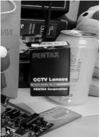
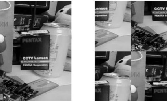
跟踪器的流程简单,并且不包括任何用于故障检测或运动建模的启发式方法。在第一帧中,我们使用图像补丁在目标的初始位置训练模型。 这个补丁(patch)大于目标(target),提供一些上下文。在新的帧,我们检测前一个位置的补丁,并将目标位置更新为产生最大值的那个。 最后,我们在新位置训练一个新模型,并将得到的α和x值与前一帧的值进行线性插值,为跟踪器提供一些记忆。
α
=
(
K
+
λ
I
)
−
1
y
\alpha=(K+\lambda I)^{-1} \mathtt {y}
α=(K+λI)−1y
α
^
=
y
^
k
^
x
x
+
λ
\hat \alpha=\frac{\hat \mathtt y}{\hat {\mathtt k}^{\mathtt {xx}}+\lambda}
α^=k^xx+λy^
(1)本文利用任何循环矩阵可以被傅里叶矩阵对角化等性质,将矩阵的运算转化为向量的Hadamad积,即元素的点乘,降低了计算量,提高运算速度,使算法满足实时性要求。
(2)将线性空间的领回归通过核函数映射到非线性空间,在非线性空间通过求解一个对偶问题和某些常见的约束,同样的可以使用循环矩阵傅里叶空间对角化简化计算。
(3)加入多通道HOG特征来代替单通道原始像素特征,提高实验的数据。
cell 越小采样越多约精确但速度慢
yf是固定的;
kf = fft2(exp(-1 / sigma^2 * max(0, (xx + yy - 2 * xy) / numel(xf))));
和如下是等价的
kf = fft2(exp(-1 / sigma^2 * abs(xx + yy - 2 * xy) / numel(xf)));

KCF 代码详解:
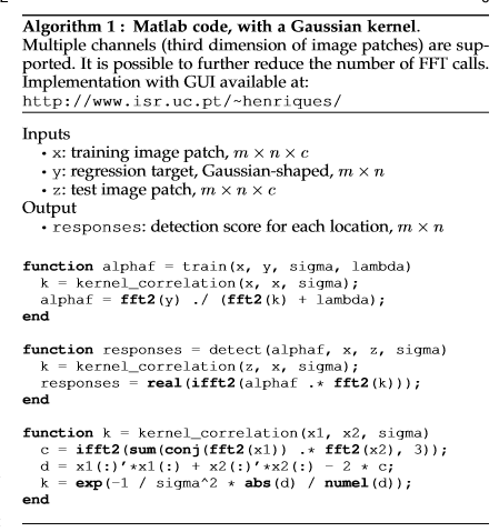
Algorithm 1 : Matlab code, with a Gaussian kernel. Multiple channels (third dimension of image patches) are supported. It is possible to further reduce the number of FFT calls. Implementation with GUI available at: https://www.isr.uc.pt/~henriques/
Inputs
•x: training image patch, m×n×c
•y: regression target, Gaussian-shaped, m×n
•z: test image patch, m×n×c
Output
•responses: detection score for each location, m×n
function alphaf = train(x, y, sigma, lambda)
  k = kernel_correlation(x, x, sigma);
  alphaf = fft2(y) ./ (fft2(k) + lambda);
end
train:
(17)
α
^
=
y
^
k
^
x
x
+
λ
\hat \alpha=\frac{\hat \mathtt y}{\hat {\mathtt k}^{\mathtt {xx}}+\lambda}{\tag {17}}
α^=k^xx+λy^(17)
function responses = detect(alphaf, x, z, sigma)
  k = kernel_correlation(z, x, sigma);
  responses = real(ifft2(alphaf .* fft2(k)));
end
detect:
(22)
f
^
(
z
)
=
k
^
x
x
⊙
α
^
\hat f(z)={\hat {\mathtt k}^{\mathtt {xx}} \odot{\hat \alpha}}{\tag {22}}
f^(z)=k^xx⊙α^(22)
function k = kernel_correlation(x1, x2, sigma)
  c = ifft2(sum(conj(fft2(x1)) .* fft2(x2), 3));
  d = x1(:)’*x1(:) + x2(:)’*x2(:) - 2 * c;
  k = exp(-1 / sigma^2 * abs(d) / numel(d));
end
kernel_correlation:
(31)
k
^
x
x
′
=
e
x
p
(
−
1
σ
(
∣
∣
x
∣
∣
2
+
∣
∣
x
′
∣
∣
2
−
2
F
−
1
(
∑
c
x
^
c
∗
⊙
x
^
c
′
)
)
)
\hat k^{\mathtt {xx\prime}}= exp(-\frac{1}{\sigma}(||\mathtt x||^2+||\mathtt x^{\prime} ||^2-2 F^{-1} (\sum_c{\hat \mathtt x^{*}_c\odot \hat \mathtt x^{\prime}_c }))){\tag {31}}
k^xx′=exp(−σ1(∣∣x∣∣2+∣∣x′∣∣2−2F−1(c∑x^c∗⊙x^c′)))(31)
matlab 画热力图:
hom=HeatMap(b);
hom=HeatMap(flipud(b));

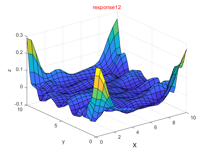
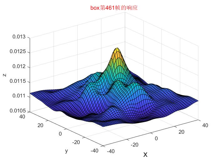
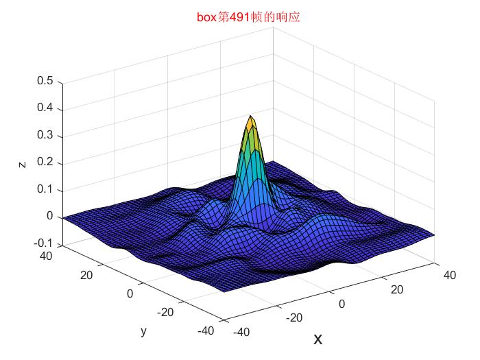
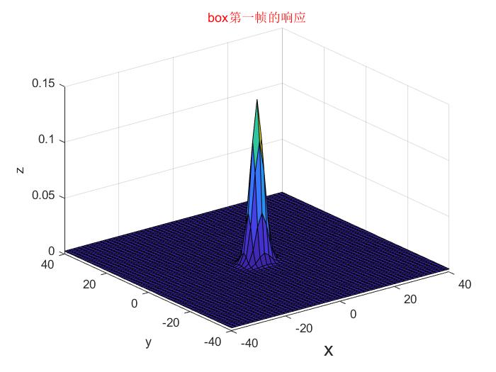
文中提到如果如果目标没有移动,峰值将会出现在左上角,而不是中心,响应在边界回荡
此时vert_delta=1, horiz_delta=1一直保持;从而不更新位置;
find(x=9)%传出x中所有x=9的点的坐标
find(x=9,1)%%传出x中的第一个等于9的点的坐标
%target location is at the maximum response. we must take into
%account the fact that, if the target doesn't move, the peak
%will appear at the top-left corner, not at the center (this is
%discussed in the paper). the responses wrap around cyclically.
[vert_delta, horiz_delta] = find(response == max(response(:)), 1);
if vert_delta > size(zf,1) / 2,  %wrap around to negative half-space of vertical axis
   vert_delta = vert_delta - size(zf,1);
end
if horiz_delta > size(zf,2) / 2,  %same for horizontal axis
	horiz_delta = horiz_delta - size(zf,2);
end
pos = pos + cell_size * [vert_delta - 1, horiz_delta - 1];
ZC = conj(Z) 返回z的复共轭
strcmp(S1,S2) 寻找S1和S2是否完全匹配,S1和S2没有顺序的区分。
matlab中single函数把一个矩阵中所有元素都变为单精度的。在matlab的命令窗口中输入doc single或者help single就可以获得函数的帮助信息
size(A, 2)表示取矩阵A的列数。如果A是多维矩阵,则表示的仍然是取每个二维矩阵的列数。
bsxfun(fun,A,B)
它的作用是:对两个矩阵A和B之间的每一个元素进行指定的计算(函数fun指定);并且具有自动扩维的作用
fun=@times 即相乘
fun=@minus 即minuus
gradientMex干嘛用的?
没有单独讲的,直接看fhog.m干嘛用的
fhog.m注释:
% Efficiently compute Felzenszwalb's HOG (FHOG) features.
%
% A fast implementation of the HOG variant used by Felzenszwalb et al.
% in their work on discriminatively trained deformable part models.
%  http://www.cs.berkeley.edu/~rbg/latent/index.html
% Gives nearly identical results to features.cc in code release version 5
% but runs 4x faster (over 125 fps on VGA color images).
%
% The computed HOG features are 3*nOrients+5 dimensional. There are
% 2*nOrients contrast sensitive orientation channels, nOrients contrast
% insensitive orientation channels, 4 texture channels and 1 all zeros
% channel (used as a 'truncation' feature). Using the standard value of
% nOrients=9 gives a 32 dimensional feature vector at each cell. This
% variant of HOG, refered to as FHOG, has been shown to achieve superior
% performance to the original HOG features. For details please refer to
% work by Felzenszwalb et al. (see link above).
%
% This function is essentially a wrapper for calls to gradientMag()
% and gradientHist(). Specifically, it is equivalent to the following:
%  [M,O] = gradientMag( I,0,0,0,1 ); softBin = -1; useHog = 2;
%  H = gradientHist(M,O,binSize,nOrients,softBin,useHog,clip);
% See gradientHist() for more general usage.
%
% This code requires SSE2 to compile and run (most modern Intel and AMD
% processors support SSE2). Please see: http://en.wikipedia.org/wiki/SSE2.
%
% USAGE
%  H = fhog( I, [binSize], [nOrients], [clip], [crop] )
%
% INPUTS
%  I        - [hxw] color or grayscale input image (must have type single)
%  binSize  - [8] spatial bin size
%  nOrients - [9] number of orientation bins
%  clip     - [.2] value at which to clip histogram bins
%  crop     - [0] if true crop boundaries
%
% OUTPUTS
%  H        - [h/binSize w/binSize nOrients*3+5] computed hog features
%
% EXAMPLE
%  I=imResample(single(imread('peppers.png'))/255,[480 640]);
%  tic, for i=1:100, H=fhog(I,8,9); end; disp(100/toc) % >125 fps
%  figure(1); im(I); V=hogDraw(H,25,1); figure(2); im(V)
%
% EXAMPLE
%  % comparison to features.cc (requires DPM code release version 5)
%  I=imResample(single(imread('peppers.png'))/255,[480 640]); Id=double(I);
%  tic, for i=1:100, H1=features(Id,8); end; disp(100/toc)
%  tic, for i=1:100, H2=fhog(I,8,9,.2,1); end; disp(100/toc)
%  figure(1); montage2(H1); figure(2); montage2(H2);
%  D=abs(H1-H2); mean(D(:))
%
% See also hog, hogDraw, gradientHist
%
% Piotr's Image&Video Toolbox      Version 3.23
% Copyright 2013 Piotr Dollar.  [pdollar-at-caltech.edu]
% Please email me if you find bugs, or have suggestions or questions!
% Licensed under the Simplified BSD License [see external/bsd.txt]

%Note: modified to be more self-contained
翻译为中文就是
有效地计算Felzenszwalb的HOG(FHOG)功能。
Felzenszwalb等人使用的HOG实现的变体。
他们在有条不紊地训练的可变形零件模型上的工作。
http://www.cs.berkeley.edu/~rbg/latent/index.html
在代码发布版本5中为features.cc提供了几乎相同的结果
但运行速度提高了4倍(VGA彩色图像超过125 fps)。
计算的HOG特征是3 * nOrients + 5维。有
2 * n对比敏感的定向通道,nOient成对比
不敏感的定向通道,4个零
channel(用作’截断’功能)。使用标准值
nOrients = 9在每个单元格处给出32维特征向量。此
HOG的变种,被称为FHOG,已被证明具有优越性
表现为原始的HOG功能。有关详细信息,请参阅
Felzenszwalb等人的工作。 (见上面的链接)。
这个函数本质上是gradientMag()的包装器
和gradientHist()。具体来说,它相当于以下内容:
[M,O] = gradientMag(I,0,0,0,1); softBin = -1; useHog = 2;
H = gradientHist(M,O,binSize,nOrients,softBin,useHog,clip);
有关更多常规用法,请参见gradientHist()。
此代码需要SSE2来编译和运行大多数(最现代的Intel和AMD)
处理器支持SSE2)。请参阅:http://en.wikipedia.org/wiki/SSE2。
注意:修改为更加独立
高斯标签函数的用法
GAUSSIAN_SHAPED_LABELS
用于样本的所有移位的高斯形标签。
LABELS = GAUSSIAN_SHAPED_LABELS(SIGMA,SZ)
为所有班次创建一系列标签
尺寸SZ的样品。 输出的大小为SZ,
每个可能的班次都有一个标签。 标签是高斯形的,
峰值在0-shift(阵列的左上角元素),衰减
随着距离的增加,并在边界处缠绕。
高斯函数具有空间带宽SIGMA。
MATLAB中的窗函数
(1)矩形窗(Rectangle Window) 调用格式:w=boxcar(n),根据长度 n 产生一个矩形窗 w。
(2)三角窗(Triangular Window) 调用格式:w=triang(n),根据长度 n 产生一个三角窗 w。
(3)汉宁窗(Hanning Window) 调用格式:w=hanning(n),根据长度 n 产生一个汉宁窗 w。
(4)海明窗(Hamming Window) 调用格式:w=hamming(n),根据长度 n 产生一个海明窗 w。
(5)布拉克曼窗(Blackman Window) 调用格式:w=blackman(n),根据长度 n 产生一个布拉克曼窗 w。
(6)恺撒窗(Kaiser Window) 调用格式:w=kaiser(n,beta),根据长度 n 和影响窗函数旁瓣的β参数产生一个恺撒窗w。
1.choose_video
function video_name = choose_video(base_path)
	%process path to make sure it's uniform
	if ispc(), base_path = strrep(base_path, '\', '/'); end
	if base_path(end) ~= '/', base_path(end+1) = '/'; end

	%list all sub-folders
	contents = dir(base_path);
	names = {};
	for k = 1:numel(contents),
		name = contents(k).name;
		if isdir([base_path name]) && ~any(strcmp(name, {'.', '..'})),
			names{end+1} = name;  %#ok
		end
	end

	%no sub-folders found
	if isempty(names), video_name = []; return; end

	%choice GUI
	choice = listdlg('ListString',names, 'Name','Choose video', 'SelectionMode','single');

	if isempty(choice),  %user cancelled
		video_name = [];
	else
		video_name = names{choice};
	end

end
2.download_video
base_path = 'D:\Datasets\kcf_data';


%list of videos to download
videos = {'basketball', 'bolt', 'boy', 'car4', 'carDark', 'carScale', ...
	'coke', 'couple', 'crossing', 'david2', 'david3', 'david', 'deer', ...
	'dog1', 'doll', 'dudek', 'faceocc1', 'faceocc2', 'fish', 'fleetface', ...
	'football', 'football1', 'freeman1', 'freeman3', 'freeman4', 'girl', ...
	'ironman', 'jogging', 'jumping', 'lemming', 'liquor', 'matrix', ...
	'mhyang', 'motorRolling', 'mountainBike', 'shaking', 'singer1', ...
	'singer2', 'skating1', 'skiing', 'soccer', 'subway', 'suv', 'sylvester', ...
	'tiger1', 'tiger2', 'trellis', 'walking', 'walking2', 'woman'};


if ~exist(base_path, 'dir')  %create if it doesn't exist already
	mkdir(base_path);
end

if ~exist('matlabpool', 'file')
	%no parallel toolbox, use a simple 'for' to iterate
	disp('Downloading videos one by one, this may take a while.')
	disp(' ')

	for k = 1:numel(videos)
		disp(['Downloading and extracting ' videos{k} '...']);
		unzip(['http://cvlab.hanyang.ac.kr/tracker_benchmark/seq/' videos{k} '.zip'], base_path);
	end

else
	%download all videos in parallel
	disp('Downloading videos in parallel, this may take a while.')
	disp(' ')

	if parpoolpool('size') == 0
		parpool open;
	end
	parfor k = 1:numel(videos)
		disp(['Downloading and extracting ' videos{k} '...']);
		unzip(['http://cvlab.hanyang.ac.kr/tracker_benchmark/seq/' videos{k} '.zip'], base_path);
	end
end
3.external.txt
NOTE: The following files are part of Piotr's Toolbox, and are provided for
convenience only:

  fhog.m
  gradientMex.mexa64
  gradientMex.mexw64

You are encouraged to get the full version of this excellent library, at which
point they can be safely deleted.
4.fhog
function H = fhog( I, binSize, nOrients, clip, crop )

if( nargin<2 ), binSize=8; end
if( nargin<3 ), nOrients=9; end
if( nargin<4 ), clip=.2; end
if( nargin<5 ), crop=0; end

softBin = -1; useHog = 2; b = binSize;

[M,O]=gradientMex('gradientMag',I,0,1);

H = gradientMex('gradientHist',M,O,binSize,nOrients,softBin,useHog,clip);

if( crop ), e=mod(size(I),b)<b/2; H=H(2:end-e(1),2:end-e(2),:); end

end
4.gaussian_correlation
function kf = gaussian_correlation(xf, yf, sigma)
%GAUSSIAN_CORRELATION Gaussian Kernel at all shifts, i.e. kernel correlation.
%   Evaluates a Gaussian kernel with bandwidth SIGMA for all relative
%   shifts between input images X and Y, which must both be MxN. They must
%   also be periodic (ie., pre-processed with a cosine window). The result
%   is an MxN map of responses.
%
%   Inputs and output are all in the Fourier domain.
%
%   Joao F. Henriques, 2014
%   http://www.isr.uc.pt/~henriques/

	N = size(xf,1) * size(xf,2);
	xx = xf(:)' * xf(:) / N;  %squared norm of x
	yy = yf(:)' * yf(:) / N;  %squared norm of y

	%cross-correlation term in Fourier domain
	xyf = xf .* conj(yf);
	xy = sum(real(ifft2(xyf)), 3);  %to spatial domain

	%calculate gaussian response for all positions, then go back to the
	%Fourier domain
	kf = fft2(exp(-1 / sigma^2 * max(0, (xx + yy - 2 * xy) / numel(xf))));

end
5.gaussian_shaped_labels
function labels = gaussian_shaped_labels(sigma, sz)
	%evaluate a Gaussian with the peak at the center element
	[rs, cs] = ndgrid((1:sz(1)) - floor(sz(1)/2), (1:sz(2)) - floor(sz(2)/2));
	labels = exp(-0.5 / sigma^2 * (rs.^2 + cs.^2));

	%move the peak to the top-left, with wrap-around
	labels = circshift(labels, -floor(sz(1:2) / 2) + 1);

	%sanity check: make sure it's really at top-left
	assert(labels(1,1) == 1)
end
6.get_features
function x = get_features(im, features, cell_size, cos_window)
	if features.hog,
		%HOG features, from Piotr's Toolbox
		x = double(fhog(single(im) / 255, cell_size, features.hog_orientations));
		x(:,:,end) = [];  %remove all-zeros channel ("truncation feature")
	end
	if features.gray,
		%gray-level (scalar feature)
		x = double(im) / 255;

		x = x - mean(x(:));
	end

	%process with cosine window if needed
	if ~isempty(cos_window),
		x = bsxfun(@times, x, cos_window);
	end

end
8.get_subwindow
function out = get_subwindow(im, pos, sz)
	if isscalar(sz),  %square sub-window
		sz = [sz, sz];
	end
	xs = floor(pos(2)) + (1:sz(2)) - floor(sz(2)/2);
	ys = floor(pos(1)) + (1:sz(1)) - floor(sz(1)/2);
	%check for out-of-bounds coordinates, and set them to the values at
	%the borders
	xs(xs < 1) = 1;
	ys(ys < 1) = 1;
	xs(xs > size(im,2)) = size(im,2);
	ys(ys > size(im,1)) = size(im,1);

	%extract image
	out = im(ys, xs, :);

end
9.linear_correlation
function kf = linear_correlation(xf, yf)
	%cross-correlation term in Fourier domain
	kf = sum(xf .* conj(yf), 3) / numel(xf);
end
10.load_video_info
function [img_files, pos, target_sz, ground_truth, video_path] = load_video_info(base_path, video)
	%see if there's a suffix, specifying one of multiple targets, for
	%example the dot and number in 'Jogging.1' or 'Jogging.2'.
	if numel(video) >= 2 && video(end-1) == '.' && ~isnan(str2double(video(end))),
		suffix = video(end-1:end);  %remember the suffix
		video = video(1:end-2);  %remove it from the video name
	else
		suffix = '';
	end

	%full path to the video's files
	if base_path(end) ~= '/' && base_path(end) ~= '\',
		base_path(end+1) = '/';
	end
	video_path = [base_path video '/'];

	%try to load ground truth from text file (Benchmark's format)
	filename = [video_path 'groundtruth_rect' suffix '.txt'];
	f = fopen(filename);
	assert(f ~= -1, ['No initial position or ground truth to load ("' filename '").'])

	%the format is [x, y, width, height]
	try
		ground_truth = textscan(f, '%f,%f,%f,%f', 'ReturnOnError',false);
	catch  %#ok, try different format (no commas)
		frewind(f);
		ground_truth = textscan(f, '%f %f %f %f');
	end
	ground_truth = cat(2, ground_truth{:});
	fclose(f);

	%set initial position and size
	target_sz = [ground_truth(1,4), ground_truth(1,3)];
	pos = [ground_truth(1,2), ground_truth(1,1)] + floor(target_sz/2);

	if size(ground_truth,1) == 1,
		%we have ground truth for the first frame only (initial position)
		ground_truth = [];
	else
		%store positions instead of boxes
		ground_truth = ground_truth(:,[2,1]) + ground_truth(:,[4,3]) / 2;
	end


	%from now on, work in the subfolder where all the images are
	video_path = [video_path 'img/'];

	%for these sequences, we must limit ourselves to a range of frames.
	%for all others, we just load all png/jpg files in the folder.
	frames = {'David', 300, 770;
			  'Football1', 1, 74;
			  'Freeman3', 1, 460;
			  'Freeman4', 1, 283};

	idx = find(strcmpi(video, frames(:,1)));

	if isempty(idx),
		%general case, just list all images
		img_files = dir([video_path '*.png']);
		if isempty(img_files),
			img_files = dir([video_path '*.jpg']);
			assert(~isempty(img_files), 'No image files to load.')
		end
		img_files = sort({img_files.name});
	else
		%list specified frames. try png first, then jpg.
		if exist(sprintf('%s%04i.png', video_path, frames{idx,2}), 'file'),
			img_files = num2str((frames{idx,2} : frames{idx,3})', '%04i.png');

		elseif exist(sprintf('%s%04i.jpg', video_path, frames{idx,2}), 'file'),
			img_files = num2str((frames{idx,2} : frames{idx,3})', '%04i.jpg');

		else
			error('No image files to load.')
		end

		img_files = cellstr(img_files);
	end

end
11.polynomial_correlation
function kf = polynomial_correlation(xf, yf, a, b)
	%cross-correlation term in Fourier domain
	xyf = xf .* conj(yf);
	xy = sum(real(ifft2(xyf)), 3);  %to spatial domain

	%calculate polynomial response for all positions, then go back to the
	%Fourier domain
	kf = fft2((xy / numel(xf) + a) .^ b);

end
12.precision_plot
function precisions = precision_plot(positions, ground_truth, title, show)
	max_threshold = 50;  %used for graphs in the paper
	precisions = zeros(max_threshold, 1);

	if size(positions,1) ~= size(ground_truth,1),
% 		fprintf('%12s - Number of ground truth frames does not match number of tracked frames.\n', title)

		%just ignore any extra frames, in either results or ground truth
		n = min(size(positions,1), size(ground_truth,1));
		positions(n+1:end,:) = [];
		ground_truth(n+1:end,:) = [];
	end

	%calculate distances to ground truth over all frames
	distances = sqrt((positions(:,1) - ground_truth(:,1)).^2 + ...
				 	 (positions(:,2) - ground_truth(:,2)).^2);
	distances(isnan(distances)) = [];

	%compute precisions
	for p = 1:max_threshold,
		precisions(p) = nnz(distances <= p) / numel(distances);
	end

	%plot the precisions
	if show == 1,
		figure('UserData','off', 'Name',['Precisions - ' title])
		plot(precisions, 'k-', 'LineWidth',2)
		xlabel('Threshold'), ylabel('Precision')
	end

end
13.run_tracker
function [precision, fps] = run_tracker(video, kernel_type, feature_type, show_visualization, show_plots)

	%path to the videos (you'll be able to choose one with the GUI).
	base_path = 'D:\Datasets\kcf_data';

	%default settings
	if nargin < 1, video = 'choose'; end
	if nargin < 2, kernel_type = 'gaussian'; end
	if nargin < 3, feature_type = 'hog'; end
	if nargin < 4, show_visualization = ~strcmp(video, 'all'); end
	if nargin < 5, show_plots = ~strcmp(video, 'all'); end


	%parameters according to the paper. at this point we can override
	%parameters based on the chosen kernel or feature type
	kernel.type = kernel_type;

	features.gray = false;
	features.hog = false;

	padding = 1.5;  %extra area surrounding the target
	lambda = 1e-4;  %regularization
	output_sigma_factor = 0.1;  %spatial bandwidth (proportional to target)

	switch feature_type
	case 'gray',
		interp_factor = 0.075;  %linear interpolation factor for adaptation

		kernel.sigma = 0.2;  %gaussian kernel bandwidth

		kernel.poly_a = 1;  %polynomial kernel additive term
		kernel.poly_b = 7;  %polynomial kernel exponent

		features.gray = true;
		cell_size = 1;

	case 'hog',
		interp_factor = 0.02;

		kernel.sigma = 0.5;

		kernel.poly_a = 1;
		kernel.poly_b = 9;

		features.hog = true;
		features.hog_orientations = 9;
		cell_size = 4;

	otherwise
		error('Unknown feature.')
	end


	assert(any(strcmp(kernel_type, {'linear', 'polynomial', 'gaussian'})), 'Unknown kernel.')


	switch video
	case 'choose',
		%ask the user for the video, then call self with that video name.
		video = choose_video(base_path);
		if ~isempty(video),
			[precision, fps] = run_tracker(video, kernel_type, ...
				feature_type, show_visualization, show_plots);

			if nargout == 0,  %don't output precision as an argument
				clear precision
			end
		end


	case 'all',
		%all videos, call self with each video name.

		%only keep valid directory names
		dirs = dir(base_path);
		videos = {dirs.name};
		videos(strcmp('.', videos) | strcmp('..', videos) | ...
			strcmp('anno', videos) | ~[dirs.isdir]) = [];

		%the 'Jogging' sequence has 2 targets, create one entry for each.
		%we could make this more general if multiple targets per video
		%becomes a common occurence.
		videos(strcmpi('Jogging', videos)) = [];
		videos(end+1:end+2) = {'Jogging.1', 'Jogging.2'};

		all_precisions = zeros(numel(videos),1);  %to compute averages
		all_fps = zeros(numel(videos),1);

		if ~exist('matlabpool', 'file'),
			%no parallel toolbox, use a simple 'for' to iterate
			for k = 1:numel(videos),
				[all_precisions(k), all_fps(k)] = run_tracker(videos{k}, ...
					kernel_type, feature_type, show_visualization, show_plots);
			end
		else
			%evaluate trackers for all videos in parallel
			if parpool('size') == 0,
				parpool open;
			end
			parfor k = 1:numel(videos),
				[all_precisions(k), all_fps(k)] = run_tracker(videos{k}, ...
					kernel_type, feature_type, show_visualization, show_plots);
			end
		end

		%compute average precision at 20px, and FPS
		mean_precision = mean(all_precisions);
		fps = mean(all_fps);
		fprintf('\nAverage precision (20px):% 1.3f, Average FPS:% 4.2f\n\n', mean_precision, fps)
		if nargout > 0,
			precision = mean_precision;
		end


	case 'benchmark',
		%running in benchmark mode - this is meant to interface easily
		%with the benchmark's code.

		%get information (image file names, initial position, etc) from
		%the benchmark's workspace variables
		seq = evalin('base', 'subS');
		target_sz = seq.init_rect(1,[4,3]);
		pos = seq.init_rect(1,[2,1]) + floor(target_sz/2);
		img_files = seq.s_frames;
		video_path = [];

		%call tracker function with all the relevant parameters
		positions = tracker(video_path, img_files, pos, target_sz, ...
			padding, kernel, lambda, output_sigma_factor, interp_factor, ...
			cell_size, features, false);

		%return results to benchmark, in a workspace variable
		rects = [positions(:,2) - target_sz(2)/2, positions(:,1) - target_sz(1)/2];
		rects(:,3) = target_sz(2);
		rects(:,4) = target_sz(1);
		res.type = 'rect';
		res.res = rects;
		assignin('base', 'res', res);


	otherwise
		%we were given the name of a single video to process.

		%get image file names, initial state, and ground truth for evaluation
		[img_files, pos, target_sz, ground_truth, video_path] = load_video_info(base_path, video);


		%call tracker function with all the relevant parameters
		[positions, time] = tracker(video_path, img_files, pos, target_sz, ...
			padding, kernel, lambda, output_sigma_factor, interp_factor, ...
			cell_size, features, show_visualization);


		%calculate and show precision plot, as well as frames-per-second
		precisions = precision_plot(positions, ground_truth, video, show_plots);
		fps = numel(img_files) / time;

		fprintf('%12s - Precision (20px):% 1.3f, FPS:% 4.2f\n', video, precisions(20), fps)

		if nargout > 0,
			%return precisions at a 20 pixels threshold
			precision = precisions(20);
		end

	end
end
14.show_video
function update_visualization_func = show_video(img_files, video_path, resize_image)
	%store one instance per frame
	num_frames = numel(img_files);
	boxes = cell(num_frames,1);

	%create window
	[fig_h, axes_h, unused, scroll] = videofig(num_frames, @redraw, [], [], @on_key_press);  %#ok, unused outputs
	set(fig_h, 'UserData','off', 'Name', ['Tracker - ' video_path])
	axis off;

	%image and rectangle handles start empty, they are initialized later
	im_h = [];
	rect_h = [];
    fps_h =[];%show the frame number
    img=[];%show color image;

	update_visualization_func = @update_visualization;
	stop_tracker = false;


	function stop = update_visualization(frame, box)
		%store the tracker instance for one frame, and show it. returns
		%true if processing should stop (user pressed 'Esc').
		boxes{frame} = box;
		scroll(frame);
		stop = stop_tracker;
	end

	function redraw(frame)

		%render main image
		im = imread([video_path img_files{frame}]);
        img = im;%show color image
		if size(im,3) > 1,
			im = rgb2gray(im);
		end
		if resize_image,
			im = imresize(im, 0.5);
		end

		if isempty(im_h),  %create image
			im_h = imshow(img, 'Border','tight', 'InitialMag',200, 'Parent',axes_h);
		else  %just update it
			set(im_h, 'CData', img)
        end

		%show the frame number
        if isempty(fps_h),
            fps_h=text('Position',[5,18], 'String','#1','Color','y', 'FontWeight','bold', 'FontSize',20,'Parent',axes_h);
        end

		%render target bounding box for this frame
		if isempty(rect_h)  %create it for the first time
			rect_h = rectangle('Position',[0,0,1,1], 'EdgeColor','g', 'Parent',axes_h);
		end
		if ~isempty(boxes{frame})
			set(rect_h, 'Visible', 'on', 'Position', boxes{frame});
            set(fps_h,'String',strcat('#',num2str(frame)));%show the frame number
		else
			set(rect_h, 'Visible', 'off');
		end
	end

	function on_key_press(key)
		if strcmp(key, 'escape')  %stop on 'Esc'
			stop_tracker = true;
		end
	end

end
15.tracker
function [positions, time] = tracker(video_path, img_files, pos, target_sz, ...
	padding, kernel, lambda, output_sigma_factor, interp_factor, cell_size, ...
	features, show_visualization)

	%if the target is large, lower the resolution, we don't need that much
	%detail
	resize_image = (sqrt(prod(target_sz)) >= 100);  %diagonal size >= threshold
	if resize_image,
		pos = floor(pos / 2);
		target_sz = floor(target_sz / 2);
	end


	%window size, taking padding into account
	window_sz = floor(target_sz * (1 + padding));

% 	%we could choose a size that is a power of two, for better FFT
% 	%performance. in practice it is slower, due to the larger window size.
% 	window_sz = 2 .^ nextpow2(window_sz);


	%create regression labels, gaussian shaped, with a bandwidth
	%proportional to target size
	output_sigma = sqrt(prod(target_sz)) * output_sigma_factor / cell_size;
	yf = fft2(gaussian_shaped_labels(output_sigma, floor(window_sz / cell_size)));

	%store pre-computed cosine window
	cos_window = hann(size(yf,1)) * hann(size(yf,2))';


	if show_visualization,  %create video interface
		update_visualization = show_video(img_files, video_path, resize_image);
	end


	%note: variables ending with 'f' are in the Fourier domain.

	time = 0;  %to calculate FPS
	positions = zeros(numel(img_files), 2);  %to calculate precision

	for frame = 1:numel(img_files),
		%load image
		im = imread([video_path img_files{frame}]);
		if size(im,3) > 1,
			im = rgb2gray(im);
		end
		if resize_image,
			im = imresize(im, 0.5);
		end

		tic()

		if frame > 1,
			%obtain a subwindow for detection at the position from last
			%frame, and convert to Fourier domain (its size is unchanged)
			patch = get_subwindow(im, pos, window_sz);
			zf = fft2(get_features(patch, features, cell_size, cos_window));

			%calculate response of the classifier at all shifts
			switch kernel.type
			case 'gaussian',
				kzf = gaussian_correlation(zf, model_xf, kernel.sigma);
			case 'polynomial',
				kzf = polynomial_correlation(zf, model_xf, kernel.poly_a, kernel.poly_b);
			case 'linear',
				kzf = linear_correlation(zf, model_xf);
			end
			response = real(ifft2(model_alphaf .* kzf));  %equation for fast detection

			%target location is at the maximum response. we must take into
			%account the fact that, if the target doesn't move, the peak
			%will appear at the top-left corner, not at the center (this is
			%discussed in the paper). the responses wrap around cyclically.
			[vert_delta, horiz_delta] = find(response == max(response(:)), 1);
			if vert_delta > size(zf,1) / 2,  %wrap around to negative half-space of vertical axis
				vert_delta = vert_delta - size(zf,1);
			end
			if horiz_delta > size(zf,2) / 2,  %same for horizontal axis
				horiz_delta = horiz_delta - size(zf,2);
			end
			pos = pos + cell_size * [vert_delta - 1, horiz_delta - 1];
		end

		%obtain a subwindow for training at newly estimated target position
		patch = get_subwindow(im, pos, window_sz);
		xf = fft2(get_features(patch, features, cell_size, cos_window));

		%Kernel Ridge Regression, calculate alphas (in Fourier domain)
		switch kernel.type
		case 'gaussian',
			kf = gaussian_correlation(xf, xf, kernel.sigma);
		case 'polynomial',
			kf = polynomial_correlation(xf, xf, kernel.poly_a, kernel.poly_b);
		case 'linear',
			kf = linear_correlation(xf, xf);
		end
		alphaf = yf ./ (kf + lambda);   %equation for fast training

		if frame == 1,  %first frame, train with a single image
			model_alphaf = alphaf;
			model_xf = xf;
		else
			%subsequent frames, interpolate model
			model_alphaf = (1 - interp_factor) * model_alphaf + interp_factor * alphaf;
			model_xf = (1 - interp_factor) * model_xf + interp_factor * xf;
		end

		%save position and timing
		positions(frame,:) = pos;
		time = time + toc();

		%visualization
		if show_visualization,
			box = [pos([2,1]) - target_sz([2,1])/2, target_sz([2,1])];
			stop = update_visualization(frame, box);
			if stop, break, end  %user pressed Esc, stop early

			drawnow
% 			pause(0.05)  %uncomment to run slower
		end

	end

	if resize_image,
		positions = positions * 2;
	end
end
16.videofig
function [fig_handle, axes_handle, scroll_bar_handles, scroll_func] = ...
	videofig(num_frames, redraw_func, play_fps, big_scroll, ...
	key_func, varargin)

	%default parameter values
	if nargin < 3 || isempty(play_fps), play_fps = 25; end  %play speed (frames per second)
	if nargin < 4 || isempty(big_scroll), big_scroll = 30; end  %page-up and page-down advance, in frames
	if nargin < 5, key_func = []; end

	%check arguments
	check_int_scalar(num_frames);
	check_callback(redraw_func);
	check_int_scalar(play_fps);
	check_int_scalar(big_scroll);
	check_callback(key_func);

	click = 0;
	f = 1;  %current frame

	%initialize figure
	fig_handle = figure('Color',[.3 .3 .3], 'MenuBar','none', 'Units','norm', ...
		'WindowButtonDownFcn',@button_down, 'WindowButtonUpFcn',@button_up, ...
		'WindowButtonMotionFcn', @on_click, 'KeyPressFcn', @key_press, ...
		'Interruptible','off', 'BusyAction','cancel', varargin{:});

	%axes for scroll bar
	scroll_axes_handle = axes('Parent',fig_handle, 'Position',[0 0 1 0.03], ...
		'Visible','off', 'Units', 'normalized');
	axis([0 1 0 1]);
	axis off

	%scroll bar
	scroll_bar_width = max(1 / num_frames, 0.01);
	scroll_handle = patch([0 1 1 0] * scroll_bar_width, [0 0 1 1], [.8 .8 .8], ...
		'Parent',scroll_axes_handle, 'EdgeColor','none', 'ButtonDownFcn', @on_click);

	%timer to play video
	play_timer = timer('TimerFcn',@play_timer_callback, 'ExecutionMode','fixedRate');

	%main drawing axes for video display
	axes_handle = axes('Position',[0 0.03 1 0.97]);

	%return handles
	scroll_bar_handles = [scroll_axes_handle; scroll_handle];
	scroll_func = @scroll;


	function key_press(src, event)  %#ok, unused arguments
		switch event.Key,  %process shortcut keys
		case 'leftarrow',
			scroll(f - 1);
		case 'rightarrow',
			scroll(f + 1);
		case 'pageup',
			if f - big_scroll < 1,  %scrolling before frame 1, stop at frame 1
				scroll(1);
			else
				scroll(f - big_scroll);
			end
		case 'pagedown',
			if f + big_scroll > num_frames,  %scrolling after last frame
				scroll(num_frames);
			else
				scroll(f + big_scroll);
			end
		case 'home',
			scroll(1);
		case 'end',
			scroll(num_frames);
		case 'return',
			play(1/play_fps)
		case 'backspace',
			play(5/play_fps)
		otherwise,
			if ~isempty(key_func),
				key_func(event.Key);  %#ok, call custom key handler
			end
		end
	end

	%mouse handler
	function button_down(src, event)  %#ok, unused arguments
		set(src,'Units','norm')
		click_pos = get(src, 'CurrentPoint');
		if click_pos(2) <= 0.03,  %only trigger if the scrollbar was clicked
			click = 1;
			on_click([],[]);
		end
	end

	function button_up(src, event)  %#ok, unused arguments
		click = 0;
	end

	function on_click(src, event)  %#ok, unused arguments
		if click == 0, return; end

		%get x-coordinate of click
		set(fig_handle, 'Units', 'normalized');
		click_point = get(fig_handle, 'CurrentPoint');
		set(fig_handle, 'Units', 'pixels');
		x = click_point(1);

		%get corresponding frame number
		new_f = floor(1 + x * num_frames);

		if new_f < 1 || new_f > num_frames, return; end  %outside valid range

		if new_f ~= f,  %don't redraw if the frame is the same (to prevent delays)
			scroll(new_f);
		end
	end

	function play(period)
		%toggle between stoping and starting the "play video" timer
		if strcmp(get(play_timer,'Running'), 'off'),
			set(play_timer, 'Period', period);
			start(play_timer);
		else
			stop(play_timer);
		end
	end
	function play_timer_callback(src, event)  %#ok
		%executed at each timer period, when playing the video
		if f < num_frames,
			scroll(f + 1);
		elseif strcmp(get(play_timer,'Running'), 'on'),
			stop(play_timer);  %stop the timer if the end is reached
		end
	end

	function scroll(new_f)
		if nargin == 1,  %scroll to another position (new_f)
			if new_f < 1 || new_f > num_frames,
				return
			end
			f = new_f;
		end

		%convert frame number to appropriate x-coordinate of scroll bar
		scroll_x = (f - 1) / num_frames;

		%move scroll bar to new position
		set(scroll_handle, 'XData', scroll_x + [0 1 1 0] * scroll_bar_width);

		%set to the right axes and call the custom redraw function
		set(fig_handle, 'CurrentAxes', axes_handle);
		redraw_func(f);

		%used to be "drawnow", but when called rapidly and the CPU is busy
		%it didn't let Matlab process events properly (ie, close figure).
		pause(0.001)
	end

	%convenience functions for argument checks
	function check_int_scalar(a)
		assert(isnumeric(a) && isscalar(a) && isfinite(a) && a == round(a), ...
			[upper(inputname(1)) ' must be a scalar integer number.']);
	end
	function check_callback(a)
		assert(isempty(a) || strcmp(class(a), 'function_handle'), ...
			[upper(inputname(1)) ' must be a valid function handle.'])
	end
end


 1558
1558


 被折叠的 条评论
为什么被折叠?
被折叠的 条评论
为什么被折叠?
 到【灌水乐园】发言


