还不会搭简单线性模型？看这里，手把手教你实现简单线性模型

本章我们通过简单线性回归模型预测黄金的价格,我们将会从数据读入、数据预处理、数据集划分、模型建立、模型效果验证等方面展开。

数据读入及预处理

from sklearn.linear_model import LinearRegression
# LinearRegression is a machine learning library for linear regression
from sklearn.linear_model import LinearRegression

# pandas and numpy are used for data manipulation
import pandas as pd
import numpy as np

# matplotlib and seaborn are used for plotting graphs
import matplotlib.pyplot as plt
%matplotlib inline
plt.style.use('seaborn-darkgrid')

# yahoo finance is used to fetch data
import yfinance as yf

# Read data
Df = yf.download('GLD', '2008-01-01', '2020-6-22', auto_adjust=True)
Df

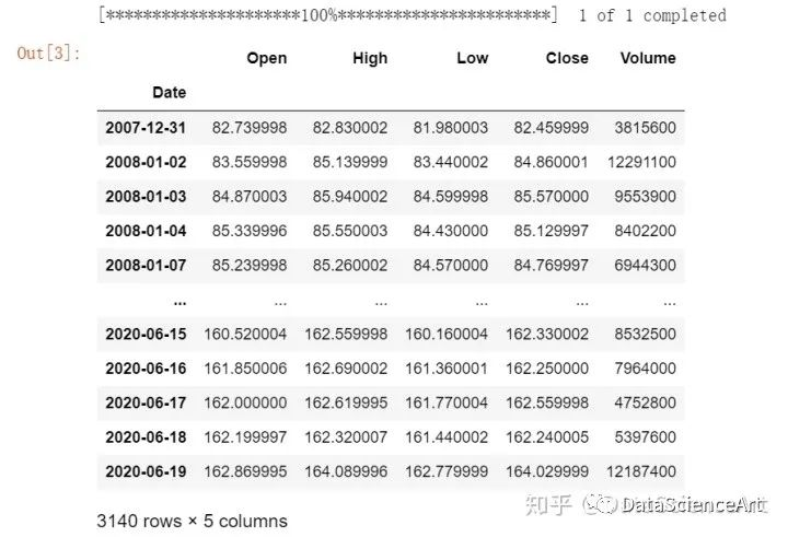
然后，我们读取了过去12年中每天黄金基金的交易信息，去除na值并且去除了黄金基金闭市时的价格的曲线。

# Only keep close columns
Df = Df[['Close']]

# Drop rows with missing values
Df = Df.dropna()

# Plot the closing price of GLD
Df.Close.plot(figsize=(10, 7),color='r')
plt.ylabel("Gold ETF Prices")
plt.title("Gold ETF Price Series")
plt.show()

定义解释变量（自变量）

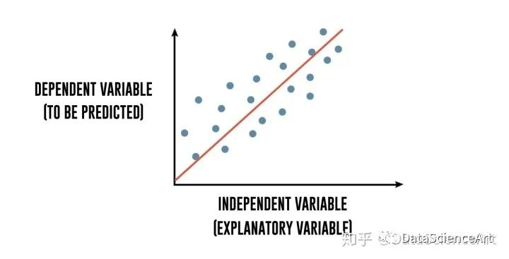
解释变量也就是我们所说的自变量，它们的值可以决定第二天Gold ETF的价格。换句话说，就是预测Gold ETF价格的特征值。在线性回归模型中，我们使用每三天以及每九天的滑动平均值作为自变量。

定义独立变量（因变量）

独立变量也就是我们所说的因变量，它的值会随着解释变量的值的改变而发生变化。

# Define explanatory variables
#rolling窗口函数，windows=3表示每三个数取一个平均值
Df['S_3'] = Df['Close'].rolling(window=3).mean()
Df['S_9'] = Df['Close'].rolling(window=9).mean()

#shift对列平移变化函数
Df['next_day_price'] = Df['Close'].shift(-1)

Df = Df.dropna()
X = Df[['S_3', 'S_9']]

# Define dependent variable
y = Df['next_day_price']
Df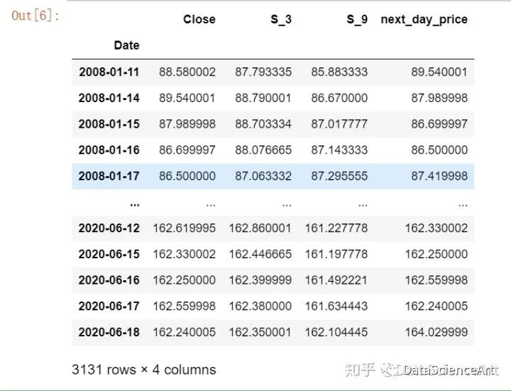

划分数据集

我们将数据集划分为训练集和测试集，训练集用来拟合线性回归模型，而测试集用来验证模型效果。

https://d1rwhvwstyk9gu.cloudfront.net/2018/01/Historical-gold-ETF.jpg

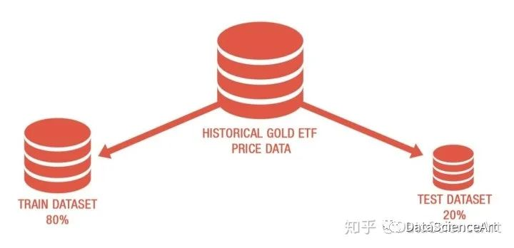
1. 80% 的数据集作为测试集，20%的数据集作为验证集

2.X_train & y_train 训练数据

3.X_test & y_test 测试数据

# Split the data into train and test dataset
t = .8
t = int(t*len(Df))

# Train dataset
X_train = X[:t]
y_train = y[:t]

# Test dataset
X_test = X[t:]
y_test = y[t:]
X_train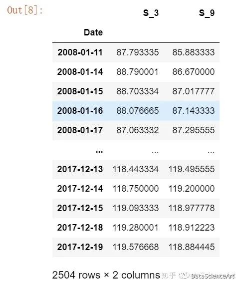

y_train

建立线性回归模型

现在，我们将创建一个线性回归模型。但是，什么是线性回归？

线性回归是利用数理统计中回归分析，来确定两种或两种以上变量间相互依赖的定量关系的一种统计分析方法，运用十分广泛。其表达形式为y = w'x+e，e为误差服从均值为0的正态分布。

回归分析中，只包括一个自变量和一个因变量，且二者的关系可用一条直线近似表示，这种回归分析称为一元线性回归分析。如果回归分析中包括两个或两个以上的自变量，且因变量和自变量之间是线性关系，则称为多元线性回归分析。

在该实例中，我们可以将线性回归模型记为以下等式：

Y = m1 X1 + m2 X2 + C

Gold ETF价格 = m1* 3天的滑动平均值+ m2 *15天的滑动平均 + c

然后我们通过fit方法去拟合X,Y。

# Create a linear regression model
linear = LinearRegression().fit(X_train, y_train)
print("Linear Regression model")
print("Gold ETF Price (y) = %.2f * 3 Days Moving Average (x1) \
+ %.2f * 9 Days Moving Average (x2) \
+ %.2f (constant)" % (linear.coef_[0], linear.coef_[1], linear.intercept_))

Output:

Linear Regression model

Gold ETF Price (y) = 1.20 3 Days Moving Average (x1) + -0.21 9 Days Moving Average (x2) + 0.43 (constant)

预测 Gold ETF价格

# Predicting the Gold ETF prices
predicted_price = linear.predict(X_test)
predicted_price = pd.DataFrame(
    predicted_price, index=y_test.index, columns=['price'])
predicted_price.plot(figsize=(10, 7))
y_test.plot()
plt.legend(['predicted_price', 'actual_price'])
plt.ylabel("Gold ETF Price")
plt.show()

我们使用  评价模型优劣。

# R square
r2_score = linear.score(X[t:], y[t:])*100
float("{0:.2f}".format(r2_score))

Output:
98.86

的取值范围在[0,100],越接近100说明模型拟合效果越好。

绘制累计收益

我们计算该策略的累积回报，以分析其效果。计算累计收益的步骤如下：生成每日金价百分比变化值，当第二天的预测价格高于当日的预测价格时，记为“ 1”表示的买入交易信号，否则记为0，将每日百分比变化乘以交易信号来计算策略收益。最后，我们将绘制累积收益图。

gold = pd.DataFrame()

gold['price'] = Df[t:]['Close']
gold['predicted_price_next_day'] = predicted_price
gold['actual_price_next_day'] = y_test
gold['gold_returns'] = gold['price'].pct_change().shift(-1)

gold['signal'] = np.where(gold.predicted_price_next_day.shift(1) < gold.predicted_price_next_day,1,0)
gold
gold['strategy_returns'] = gold.signal * gold['gold_returns']
((gold['strategy_returns']+1).cumprod()).plot(figsize=(10,7),color='g')
plt.ylabel('Cumulative Returns')
plt.show()

'Sharpe Ratio %.2f' % (gold['strategy_returns'].mean()/gold['strategy_returns'].std()*(252**0.5))

'Sharpe Ratio 0.75'

如何运用模型预测日常波动

data = yf.download('GLD', '2008-06-01', '2020-6-25', auto_adjust=True)
data['S_3'] = data['Close'].rolling(window=3).mean()
data['S_9'] = data['Close'].rolling(window=9).mean()
data = data.dropna()
data['predicted_gold_price'] = linear.predict(data[['S_3', 'S_9']])
data['signal'] = np.where(data.predicted_gold_price.shift(1) < data.predicted_gold_price,"Buy","No Position")
data.tail(7)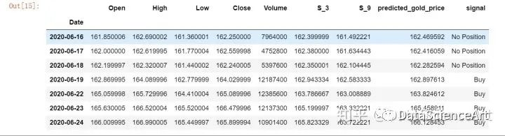

参考链接

https://blog.quantinsti.com/gold-price-prediction-using-machine-learning-python

分享、点赞、在看三连