FDTD Solutions 批量建立任意角度的监测器实现纳米粒子散射相位函数的监测（Part1-方法1）

---

前言

FDTD Solutions软件基于矢量3维麦克斯维方程求解，采用时域有限差分FDTD法将空间网格化，时间上一步步计算，从时间域信号中获得宽波段的稳态连续波结果。参考百度百科近些年，凭借其强大的性能深受研究工作者喜爱，并被广泛应用与超表面、纳米颗粒散射、太阳能电池等诸多研究领域。然而，其采用立方体晶胞的网格划分，导致软件的监测器均是平行于笛卡尔坐标轴的面监测器或立方体监测器。很多时候，我们需要观察某一角度方位上的电磁场情况，就必须 借助一定的脚本语言构建监测器组来实现。

---

提示：以下是本篇文章正文内容，下面案例可供参考，本案例主要阐述如何利用FDTD脚本语言来批量生成任意角度的点监测器，帮助大家建立这种构建监测器的思想。后续进阶文章中我会介绍利用脚本语言构建任意观测角度，任意分辨率的面监测器的方法。

一、以监测纳米粒子散射相函数为例（监测角度0-180°范围内，某一传播距离位置处的光强值）

下面直接进行建立方法的阐述

二、构建步骤

1.建立纳米粒子仿真模型

首先，打开FDTD Solutions仿真软件，新建一个工程文件(默认类型即可)，命名为 ：NanoParticlesScatter.fsp
设置球形纳米结构参数
菜单栏：Structures—Sphere

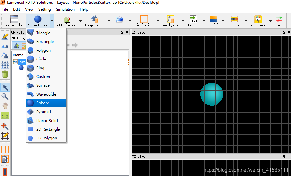
设置纳米粒子尺寸，材料等参数
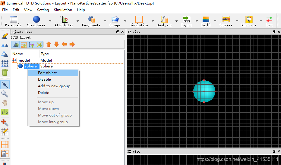
step1：目录树中右键sphere，选择Edit object
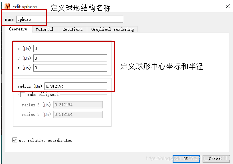
step2
step3：此处可以直接输入材料的折射率，也可以从material下拉选项中选择相应的材料

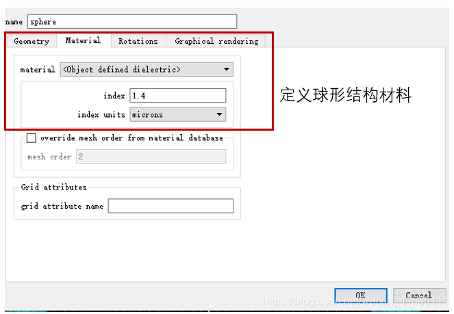
2.设置全场散射光源TFSF

设置散射场光源参数，光源范围、波长、入射和偏振方向等
step1：目录树中右键sphere，选择Edit object
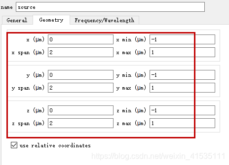
step2：各参数的含义与设置参考我上传的资源“《FDTD Solutions Reference Guide>》page52-53页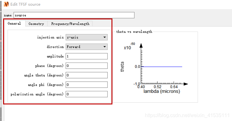step3：设置光源区域（大于球形结构区域）

step4：设置光源波长与带宽（此处以单波长400nm为例）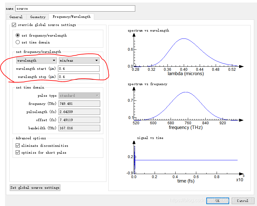

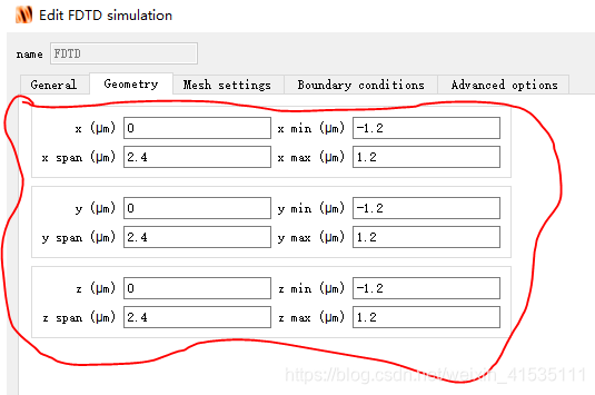
3.设置FDTD仿真区域

设置FDTD仿真区域、网格划分形式、网格精度等
step1：设置FDTD仿真区域（大于光源区域）
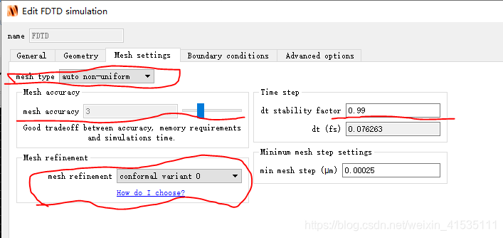
step2：FDTD选项中Mesh setting设置
mesh type：一般选择auto non-uniform，结构部分网格划分精细，非结构区域网格划分粗糙；也可以根据需要在下拉选项中选择其他网格划分形式；
mesh accuracy：仿真精度需要预先仿真测试，数值越高，仿真越精确，对计算机内存性能要求越高；可以从精度1-5依次增加，直到在某精度下，仿真结果不变，即可确定该精度已经足够满足仿真要求；
mesh refinement: 金属材料通常选择Conformal variant 1，介质材料一般Conformal variant 0，根据实际情况设置（参考该帖子）以及《FDTD Solutions Reference Guide》。
dt stability factor:在一些仿真结果不收敛的地方考虑修改
step2：本实例中FDTD选项中边界条件设置为PML

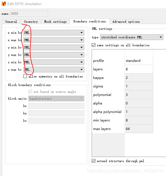
4.批量生成监测器，构建监测器组

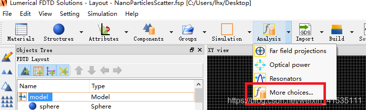
step1：在analysis选项中选择更多，在object library中插入一个分析组，分析组区域要小于FDTD区域大于光源区域，只有这样才是获得的散射场数据。
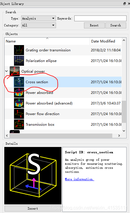
step2：如选择任意一个分析组（Cross-section）插入，删除原有的脚本内容，对该分析组脚本进行重新编辑（也可以直接插入angled monitor或者Curved monitor，本案例重点介绍脚本编辑思想，后续介绍这两个监测器组）

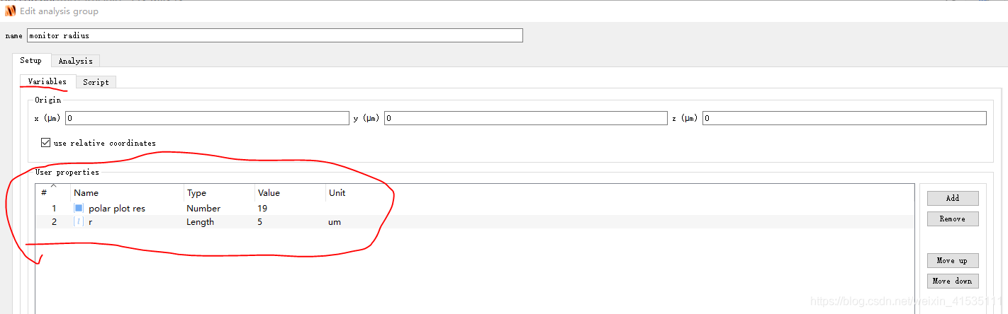
step3：利用脚本声明建模所用到的变量，构建多个点监测器

##################本部分为脚本说明############################
Angled monitor
#This script creates an effective 2D monitor by using a large
#number of point monitors.
#Monitor spatial resolution(polar plot res):
#The resolution of the data is controled by setting the number of point monitors.
#Note: As more monitors are used, the simulation time and memory requirements will increase.
#Also, there is no value in making the resolution of these monitors higher than the resolution of the main FDTD mesh.
#Input properties
#polar plot res:the number of monitors or The resolution of the data.
#r: the distance from the sphere center to the monitors.
#Copyright 2021-01-27-HXL
###################以下部分为正式脚本#######################
（注意，#表示注释部分）

deleteall;
phi = linspace(0,360,%polar plot res%); # user-modifiable in the Variables tab
npts = length(phi);
#add monitors
for(j=1:npts)
{ 
addprofile; 
set('monitor type','point');
x=r*sin(phi(j)*pi/180);#Define the X coordinate of the monitor
y=r*cos(phi(j)*pi/180);#Define the X coordinate of the monitor
set('x',x);
set('y',y);
set('z',0);
set('output Px',1);
set('output Py',1);
set('output Pz',1); 
}

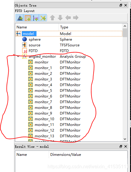
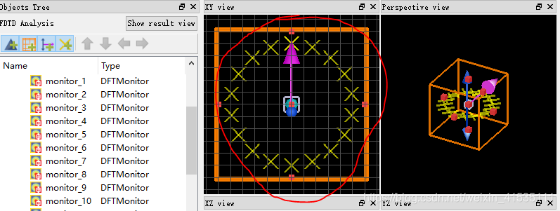
step4：分析组脚本修改运行后的监测器组效果如下

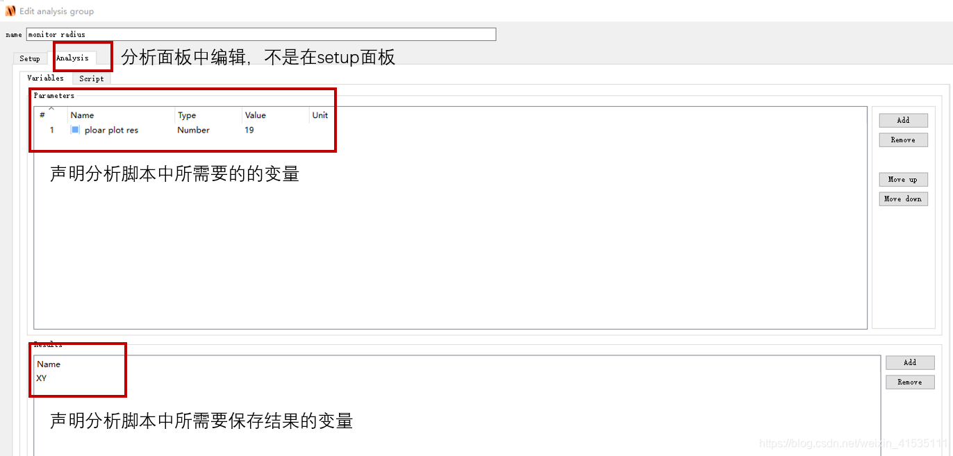
step5：声明分析所用的变量和需要保存的变量；并利用脚本分析保存多个监测器的数据

#################本部分为脚本说明###########################
#Angled monitor
#This script is used to analyze and save the datas of a large number of point monitors.
#Monitor spatial resolution(polar plot res):
#The resolution of the data is controled by setting the number of point monitors.
#Note: As more monitors are used, the simulation time and memory requirements will increase.
#Also, there is no value in making the resolution of these monitors higher than the resolution of the main FDTD mesh.
#Input properties
#polar plot res:the number of monitors or The resolution of the data.
#The value of “the polar plot res” in Analysis-Variables panel should be the same as in Setup-Variables panel.(Very important!!!)
#Copyright 2021-01-27-HXL
##################以下部分为正式脚本############################

f = getdata('monitor','f');
phi = linspace(0,360,%polar plot res%); # user-modifiable in the Variables tab
Num = length(phi);
Ex = matrix(1,Num);#Create a new empty matrix to save "Ex"
Ey = matrix(1,Num);#Create a new empty matrix to save "Ey"
Ez = matrix(1,Num);#Create a new empty matrix to save "Ez"
E2_xy = matrix(1,Num);#Create a new empty matrix to save total field 
for(i=0:Num-1)
{
    if(i==0) {
    m = 'monitor';
    if(havedata(m)){
  Ex(1,1) = getdata(m, "Ex");#Save datas of monitor
  Ey(1,1) = getdata(m, "Ey");
  Ez(1,1) = getdata(m, "Ez");}

    } else {
     m = 'monitor_' + num2str(i);
      if(havedata(m)){
  Ex(1,i+1) = getdata(m, "Ex");#Save datas of monitor_i
  Ey(1,i+1) = getdata(m, "Ey");
  Ez(1,i+1) = getdata(m, "Ez");}    
      }
  }
  
  E2_xy = abs(Ex)^2 + abs(Ey)^2 + abs(Ez)^2;#Calcaulate total field  
  #Save datas to matrix-XY and visual display
  XY = matrixdataset("XY");
  XY.addparameter("phi",phi);
  XY.addparameter("lambda",c/f,"f",f);
  XY.addattribute("E2",E2_xy);

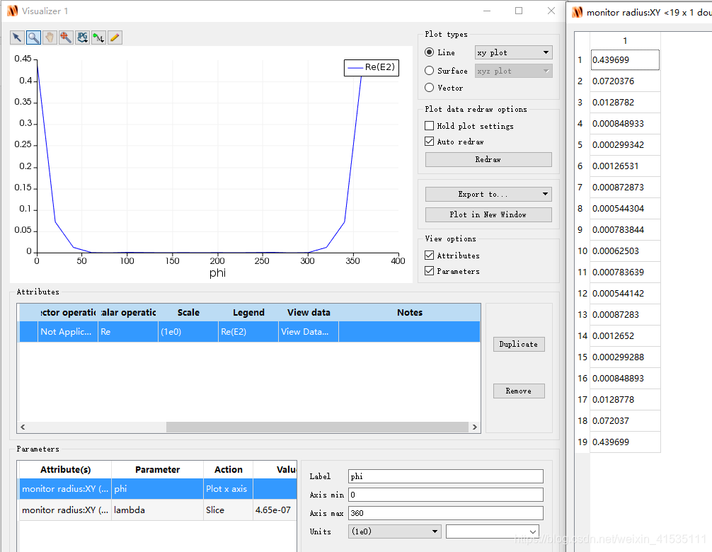
6.运行结果

7.说明与仿真模型源文件（NanoParticlesScatter.fsp）

链接中的实例参数设置可能会与前文截图中的数据不同！！！可自行查看修改。
FDTD仿真源文件下载链接