吴恩达线性回归

线性回归

导入必须的包

import pandas as pd
import matplotlib.pyplot as plt
import numpy as np

导入数据

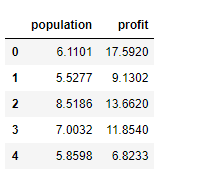
data=pd.read_csv(‘ex1data1.txt’,names=[‘population’,‘profit’])

查看信息

data.head()

插入1

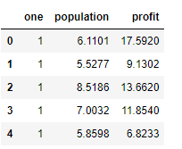
data.insert(0,‘one’,1)
data.head()

切割数据获取X，y值

cols=data.shape[1]
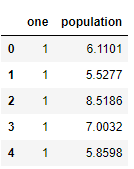
X=data.iloc[:,0:cols-1]
y=data.iloc[:,cols-1:cols]

查看X

X.head()

y.head()

转换为矩阵形式

X=np.matrix(X.values)
y=np.matrix(y.values)
theta=np.matrix(np.array([0,0]))

查看维度信息

X.shape

y.shape

theta.shape

建立代价函数

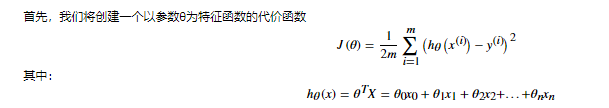
def computeCost(X,y,theta):
inner=np.power(((Xtheta.T)-y),2)
return np.sum(inner)/(2len(X))

计算代价值，未调整参数

computeCost(X,y,theta)

设置学习率 迭代次数

alpha=0.01
iters=1000

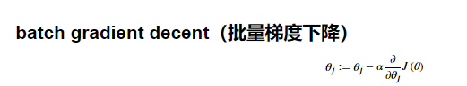
批量梯度下降

def gradientDescent(X,y,theta,alpha,iters):
temp=np.matrix(np.zeros(theta.shape))
parameters=int(theta.ravel().shape[1])
cost=np.zeros(iters)
for i in range(iters):
error=(X*theta.T)-y
for j in range(parameters):
term=np.multiply(error,X[:,j])
temp[0,j]=theta[0,j]-((alpha/len(X))*np.sum(term))
theta=temp
cost[i]=computeCost(X,y,theta)
return theta,cost

计算批量梯度下降后代价函数值

g,cost=gradientDescent(X,y,theta,alpha,iters)
computeCost(X,y,g)

特征变量小于1W也可以使用正规方程计算参数值

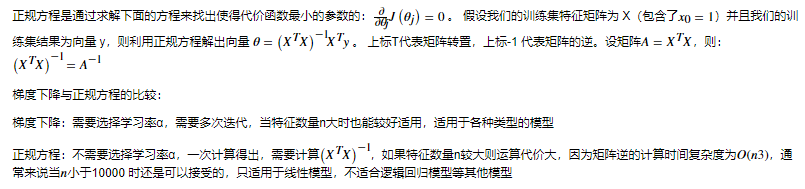
def normalEpn(X,y):
theta=np.linalg.inv(X.T@X)@X.T@y
return theta

final_theta2=normalEpn(X,y)

计算代价函数值

computeCost(X,y,final_theta2.T)