机器学习-人与机器生数据的区分模型测试-数据处理1-CSDN博客

本文链接：https://blog.csdn.net/weixin_41870426/article/details/148035943

附件为训练数据，总体的流程可以作为参考。

导入依赖

import pandas as pd
import os
import numpy as np
from sklearn.model_selection import train_test_split,GridSearchCV
from sklearn.ensemble import RandomForestClassifier,VotingClassifier 
from sklearn.metrics import accuracy_score, classification_report, confusion_matrix,roc_curve
from xgboost import XGBClassifier
from sklearn.linear_model import LogisticRegression
from sklearn.neighbors import KNeighborsClassifier
from sklearn.tree import DecisionTreeClassifier
from lightgbm import LGBMClassifier
import matplotlib.pyplot as plt
import seaborn as sns
from sklearn.preprocessing import StandardScaler,LabelEncoder
from catboost import CatBoostClassifier
from statsmodels.stats.outliers_influence import variance_inflation_factor
# 分析高频共现特征组合
from mlxtend.frequent_patterns import apriori
from sklearn.metrics import roc_auc_score
import json

# 设置工作目录
os.chdir(r'D:\python code\人工与机器人识别')
# 加载数据集
data = pd.read_csv('bots_vs_users.csv')  # 替换为你的数据集路径

EDA

数据分布

def clean_data(data):
    for col in data.columns:
        print(col)
        if col == 'city':  # 跳过第一列
            continue
        else:    
            data[col] = data[col].replace('Unknown','-1')  # 使用均值填充缺失值
            data[col] = data[col].astype('float64')  # 转换为数值类型
            data[col] = data[col].fillna(data[col].mean())  # 使用均值填充缺失值

    return data
    
data = clean_data(data)

encoder = LabelEncoder()
encoder.fit(data['city'])  # 只在第一个DF上fit
data['city2'] = encoder.transform(data['city'])


# 第一次拆分：训练集（70%） + 临时集（30%）, 
data,temp = train_test_split(data, test_size=0.1, random_state=42)


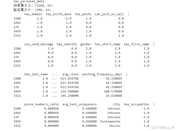
# 输出拆分后的数据集大小
print("训练集大小:", data.shape)
print("验证集大小:", temp.shape)
print(data.head())

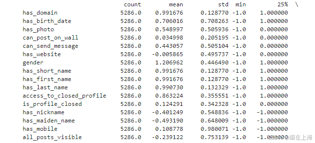
这里是数据的相关描述统计

入图片描述

描述统计

# 训练集编码
target_list = ['city', 'target', 'city2']
data_clean = data.drop(target_list, axis=1).copy()

# 基本统计描述
print(data_clean.describe().T)

print("方差:\n", data_clean.var(numeric_only=True))
print("众数:\n", data_clean.mode().T) 
print("偏度:\n", data_clean.skew(numeric_only=True))  # 需确保数据为数值型
print("峰度:\n", data_clean.kurtosis(numeric_only=True))

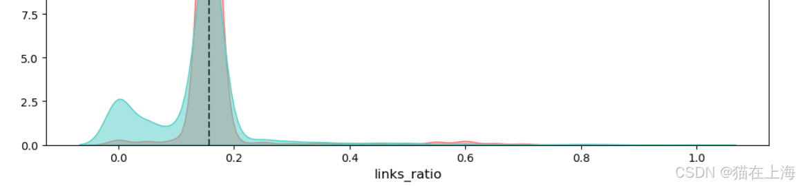
查看数据的分布情况
在这里插入图片描述


def plot_cont_var_dist(df, feature, target='target'):
    """
    绘制连续变量的正负样本核密度估计图（KDE），并计算并标注 KS（Kolmogorov-Smirnov）统计量。

    参数:
    df (pandas.DataFrame): 包含特征和目标变量的数据集。
    feature (str): 要绘制的连续特征的名称。
    target (str, 可选): 目标变量的名称，默认为 'target'。

    """
    # 设置图形的大小
    plt.figure(figsize=(10,6))
    
    # 提取正样本数据，并处理无穷大值，移除缺失值
    pos_data = df.loc[df[target]==1, feature].replace([np.inf, -np.inf], np.nan).dropna()
    # 提取负样本数据，并处理无穷大值，移除缺失值
    neg_data = df.loc[df[target]==0, feature].replace([np.inf, -np.inf], np.nan).dropna()
    
    # 绘制正样本的核密度估计图
    sns.kdeplot(pos_data, label='Positive', 
                fill=True, alpha=0.5, color='#FF6B6B')
    # 绘制负样本的核密度估计图
    sns.kdeplot(neg_data, label='Negative',
                fill=True, alpha=0.5, color='#4ECDC4')
    
    # 检查正样本或负样本数据是否为空，如果为空则跳过该特征的绘制
    if pos_data.empty or neg_data.empty:
        print(f"Skipped {feature} due to empty data")
        plt.close()
        return
    
    try:
        # 计算 ROC 曲线所需的假正率、真正率和阈值
        # 由于使用连续变量计算 KS 需要离散化处理，这里借助 roc_curve 函数
        fpr, tpr, thresholds = roc_curve(df[target], df[feature])
        # 计算 KS 统计量，即真正率与假正率差值的最大值
        ks_value = max(tpr - fpr)
        # 找到对应 KS 统计量最大值的阈值
        ks_threshold = thresholds[np.argmax(tpr - fpr)]
    except Exception as e:
        # 若计算 KS 统计量时出错，打印错误信息并关闭图形
        print(f"Error calculating KS for {feature}: {str(e)}")
        plt.close()
        return
    
    # 在图中绘制 KS 阈值对应的垂直线
    plt.axvline(ks_threshold, color='#2A363B', linestyle='--', 
                linewidth=1.5, label=f'Cutoff: {ks_threshold:.2f}')
    # 设置图形标题，包含特征名称和 KS 统计量的值
    plt.title(f'{feature}\nKS Statistic = {ks_value:.2f}', fontsize=14)
    # 设置 x 轴标签
    plt.xlabel(feature, fontsize=12)
    # 设置 y 轴标签
    plt.ylabel('Density', fontsize=12)
    # 显示图例，去掉边框
    plt.legend(frameon=False)
    # 自动调整子图参数，使之填充整个图像区域
    plt.tight_layout()
    # 显示图形
    plt.show()
    # 关闭图形，释放内存
    plt.close()

# 改进后的过滤逻辑
def is_valid_numeric(col_data):
    """
    判断传入的列数据是否为有效的数值型特征。

    有效的数值型特征需满足以下条件：
    1. 数据类型为数值类型。
    2. 唯一值的数量超过 20 个。
    3. 数据类型不是分类类型。

    参数:
    col_data (pandas.Series): 需要进行判断的列数据。

    返回:
    bool: 如果满足所有条件则返回 True，否则返回 False。
    """
    return (
        # 检查数据类型是否为数值类型
        pd.api.types.is_numeric_dtype(col_data) and 
        # 检查唯一值的数量是否超过 20 个
        col_data.nunique() > 20 and
        # 检查数据类型是否不是分类类型
        not isinstance(col_data.dtype, pd.CategoricalDtype)
    )

filtered_list = [col for col in data.columns 
                if col not in target_list and is_valid_numeric(data[col])]

# 增强型绘图循环
for col in filtered_list:
    try:
        # 预处理inf值
        data[col] = data[col].replace([np.inf, -np.inf], np.nan)
        # 跳过缺失率过高的特征
        if data[col].isnull().mean() > 0.8:
            print(f"Skipped {col} due to high missing rate")
            continue
            
        plot_cont_var_dist(data, col)
    except Exception as e:
        print(f"Plotting failed for {col}: {str(e)}")



#查看数据1的分布情况
one_ratio_list = []
for col in data.columns:
    if col == 'city' or col == 'target' or col == 'city2':  # 跳过第一列
        continue
    else:
        one_ratio = data[col].mean()  # 计算1值占比
        print(f"{col}: {one_ratio}")
        one_ratio_list.append(one_ratio)


plt.figure(figsize=(8,4))
sns.histplot(one_ratio_list, bins=20, kde=True)
plt.title('Histogram of 1-Value Proportion Distribution')
plt.xlabel('Proportion of 1 value')
plt.show()