机器学习-人与机器生数据的区分模型测试 - 模型融合与检验

模型融合

# 先用普通Pipeline训练
from sklearn.pipeline import Pipeline

#from sklearn2pmml.pipeline import PMMLPipeline
train_pipe = Pipeline([
    ('scaler', StandardScaler()),
    ('ensemble', VotingClassifier(estimators=[
        ('rf', RandomForestClassifier(n_estimators=200, max_depth=10,min_samples_split = 20)), 
        ('xgb', XGBClassifier(max_depth=4, learning_rate=0.1,n_estimators = 200 )),  
        ('lgb', LGBMClassifier(num_leaves=200,max_depth=5,learning_rate=0.1, reg_alpha=0.1,n_estimators = 200,lambda_l1 =0.1,lambda_l2=2 )),  
        ('cat', CatBoostClassifier(n_estimators=150, max_depth=10,learning_rate=0.01))
    ], voting='soft'))
])
train_pipe.fit(X_train, y_train)

数据保存与检验

import joblib
import pandas as pd
import numpy as np
import matplotlib.pyplot as plt
from sklearn.metrics import (accuracy_score, roc_auc_score, 
                           roc_curve, confusion_matrix)
                           

数据保存

# 数据保存
def save_data():
    pd.DataFrame(X_train).to_csv('X_train.csv', index=False)
    pd.DataFrame(y_train).to_csv('y_train.csv', index=False)
    pd.DataFrame(X_temp).to_csv('X_test.csv', index=False)
    pd.DataFrame(y_temp).to_csv('y_test.csv', index=False)
    joblib.dump(train_pipe, 'trained_model.pkl')

准确率比对

def compare_accuracy():
    train_pred = train_pipe.predict(X_train)
    test_pred = train_pipe.predict(X_temp)
    train_acc = accuracy_score(y_train, train_pred)
    test_acc = accuracy_score(y_temp, test_pred)
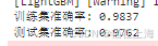
    print(f"训练集准确率: {train_acc:.4f}")
    print(f"测试集准确率: {test_acc:.4f}")

模型稳定性分析

def stability_analysis():
    # 交叉验证稳定性
    from sklearn.model_selection import cross_val_score
    cv_scores = cross_val_score(train_pipe, X_train, y_train, cv=5)
    print(f"交叉验证得分: {cv_scores}")
    print(f"平均交叉验证得分: {np.mean(cv_scores):.4f} (±{np.std(cv_scores):.4f})")
    
    # 特征重要性分析
    try:
        importances = train_pipe.named_steps['ensemble'].feature_importances_
        plt.figure()
        plt.bar(range(len(importances)), importances)
        plt.title('特征重要性')
        plt.savefig('feature_importance.png')
        plt.close()
    except AttributeError:
        print("当前集成方法不支持特征重要性分析")

最总结果

# 模型预测
y_prob = train_pipe.predict_proba(X_temp)[:, 1]
fpr, tpr, thresholds = roc_curve(y_temp, y_prob)
auc = roc_auc_score(y_temp, y_prob

# Lift值计算优化
decile = pd.DataFrame({'prob': y_prob, 'actual': y_temp})
decile['decile'] = pd.qcut(decile['prob'].rank(method='first'), 
                            10, labels=False)
lift = decile.groupby('decile')['actual'].mean() / decile['actual'].mean()


# 可视化增强
fig, (ax1, ax2) = plt.subplots(1, 2, figsize=(14, 6))

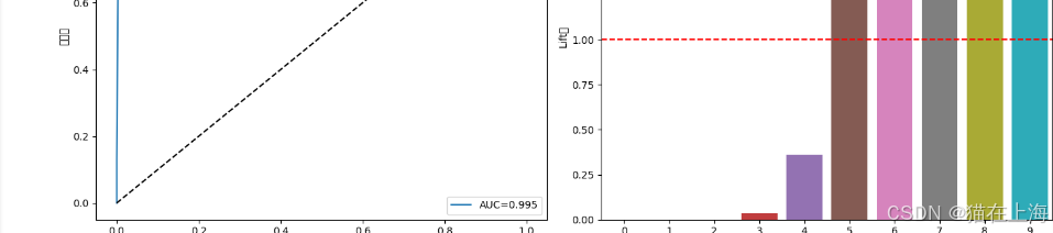
# ROC曲线
ax1.plot(fpr, tpr, label=f'AUC={auc:.3f}')
ax1.plot([0, 1], [0, 1], 'k--')
ax1.set_xlabel('假正率')
ax1.set_ylabel('真正率')
ax1.set_title('ROC曲线')
ax1.legend()

# Lift曲线
sns.barplot(x=lift.index, y=lift.values, ax=ax2)
ax2.axhline(1, color='red', linestyle='--')
ax2.set_title('Lift值分布')
ax2.set_xlabel('十分位')
ax2.set_ylabel('Lift值')

plt.tight_layout()
plt.savefig('model_performance.png', dpi=300, bbox_inches='tight')

结果如下

最后输出ROC曲线和lift 值