介绍两款生成神经网络架构示意图的工具：NN-SVG和PlotNeuralNet

对于神经网络架构的可视化是很有意义的，可以在很大程度上帮助到我们清晰直观地了解到整个架构，我们在前面的 PyTorch的ONNX结合MNIST手写数字数据集的应用(.pth和.onnx的转换与onnx运行时)
有介绍，可以将模型架构文件(常见的格式都可以)在线上传到 https://netron.app/，将会生成架构示意图，比如将yolov5s.pt这个预训练模型，上传之后，将出现下面这样的图片(局部)：

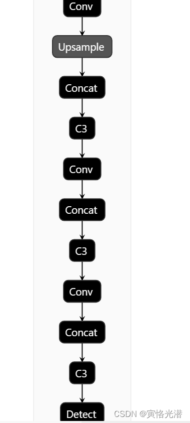
这种属于非常简单的层的连接展示，也能够直观知道整个架构是由哪些层组成，虽然每层可以查看一些属性，不过对于每层的具体细节并没有那么直观展现在图片当中。
接下来介绍的这两款都会生成漂亮的可视化神经网络图，可以用来绘制报告和演示使用，效果非常棒。 

1、NN-SVG

NN-SVG生成神经网络架构的地址：http://alexlenail.me/NN-SVG/AlexNet.html
显示可能很慢，最好科学上网，进去之后，我们可以看到，有三种神经网络架构可以进行设置：FCNN、LeNet、AlexNet 我们分别来看下：

1.1、FCNN 

第一种就是最基础的全连接神经网络FCNN，输入层-->隐藏层(若干)-->输出层，截图如下：

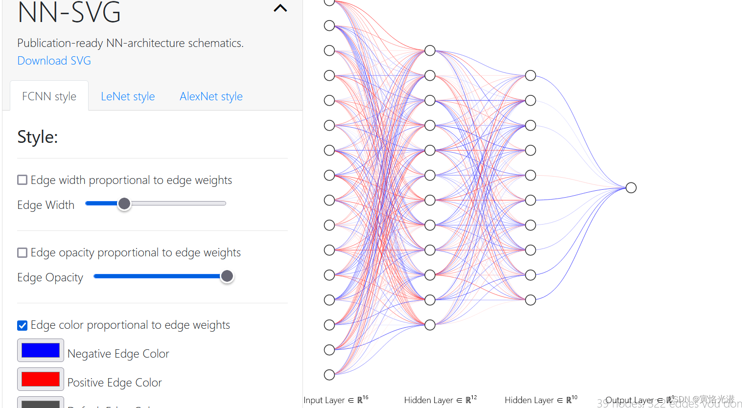
左侧边栏可以进行一些颜色、形状、透明度等设置，也可以很方便的增加和减少层。右边就会实时的显示出操作的效果。

1.2、LeNet

LeNet是一种经典的卷积神经网络，最初用来识别手写数字，我们来看下其结构：

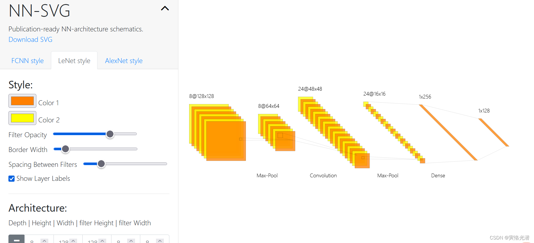
可以看到架构主要是由卷积层组成，输入层-->卷积层-->最大池化层-->...-->全连接层-->输出层。
左边同样的都是可以设置颜色，透明度等，可以增减层数，在每层里可以设置数量、高宽以及卷积核大小，还可以指定是否显示层的名称，这样就更加清楚的知道架构是由哪些具体的层组成了。

1.3、AlexNet

AlexNet是辛顿和他的学生Alex Krizhevsky设计的CNN，在2012年ImageNet的竞赛中获得冠军，它是在LeNet的基础上应用了ReLU激活函数(取代Sigmoid)、Dropout层(避免过拟合)、LRN层(增强泛化能力)等的一种神经网络，截图如下：

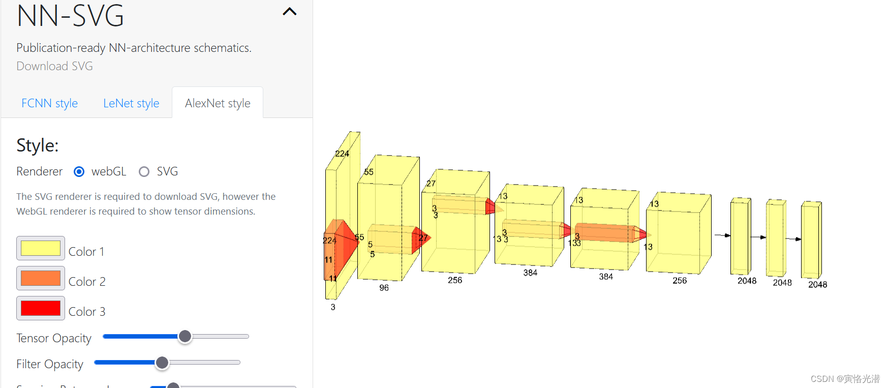
同样的可以直观看到，每个层的数量、宽高、卷积核的大小，这些直观的神经网络示意图，尤其对于初学者来说可以很好的理解某个神经网络的整个计算过程。
最后的这些都是可以点击"Download SVG"将其下载成svg格式(一种XML格式)的文件。

2、PlotNeuralNet

2.1、安装

首先确认自己的操作系统，然后对应着进行安装，后面出现的示例是本人的Ubuntu 18.04版本上做的。

Ubuntu 16.04

sudo apt-get install texlive-latex-extra

Ubuntu 18.04.2
基于本网站，请安装以下软件包，包含一些字体包：

sudo apt-get install texlive-latex-base
sudo apt-get install texlive-fonts-recommended
sudo apt-get install texlive-fonts-extra
sudo apt-get install texlive-latex-extra

Windows或其他系统

下载安装MiKTeX：https://miktex.org/download

下载安装Git bash：https://git-scm.com/download/win
或者Cygwin：https://www.cygwin.com/
准备就绪之后运行即可：

cd pyexamples/
bash ../tikzmake.sh test_simple

2.2、克隆运行

上面的Latex安装好了之后，就克隆PlotNeuralNet： 

git clone https://github.com/HarisIqbal88/PlotNeuralNet.git

 我们先来执行自带的一个测试文件

cd pyexamples/
bash ../tikzmake.sh test_simple

将生成test_simple.pdf，截图如下：

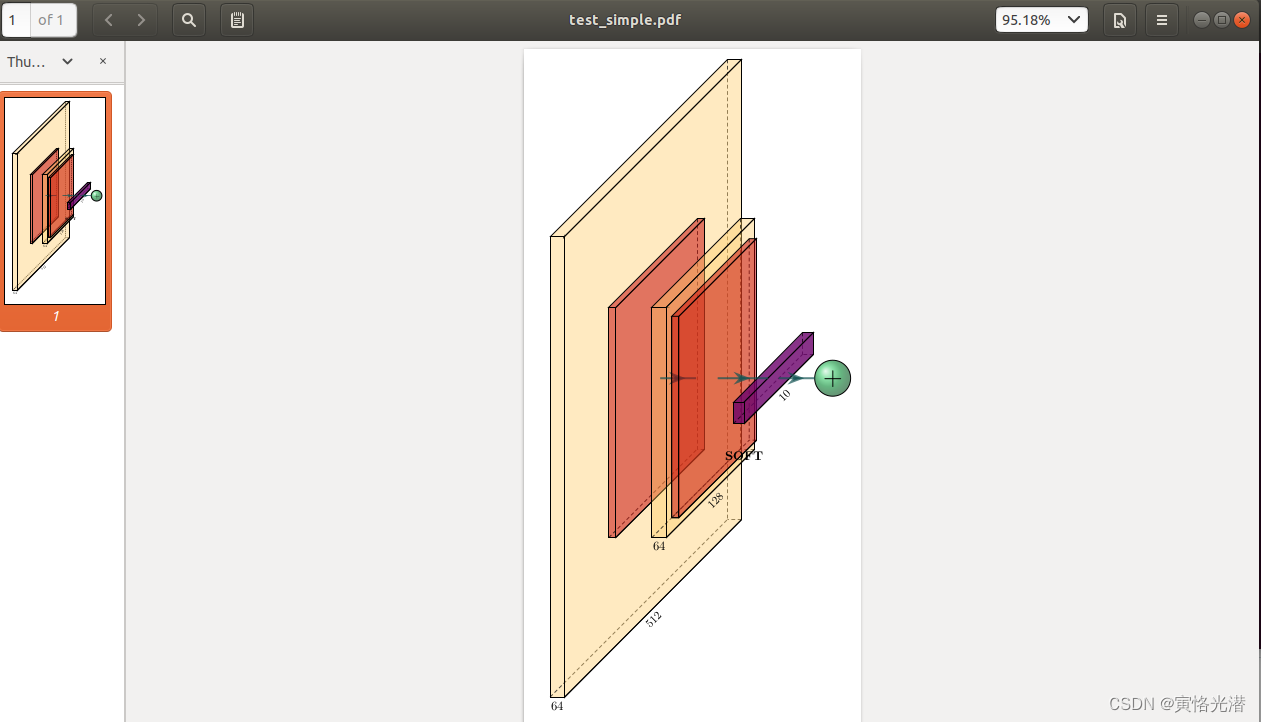
2.3、test_simple.py

我们来看下自带的test_simple.py内容：

import sys
sys.path.append('../')
from pycore.tikzeng import *

# defined your arch
arch = [
    to_head( '..' ),
    to_cor(),
    to_begin(),
    to_Conv("conv1", 512, 64, offset="(0,0,0)", to="(0,0,0)", height=64, depth=64, width=2 ),
    to_Pool("pool1", offset="(0,0,0)", to="(conv1-east)"),
    to_Conv("conv2", 128, 64, offset="(1,0,0)", to="(pool1-east)", height=32, depth=32, width=2 ),
    to_connection( "pool1", "conv2"), 
    to_Pool("pool2", offset="(0,0,0)", to="(conv2-east)", height=28, depth=28, width=1),
    to_SoftMax("soft1", 10 ,"(3,0,0)", "(pool1-east)", caption="SOFT"  ),
    to_connection("pool2", "soft1"),    
    to_Sum("sum1", offset="(1.5,0,0)", to="(soft1-east)", radius=2.5, opacity=0.6),
    to_connection("soft1", "sum1"),
    to_end()
    ]

def main():
    namefile = str(sys.argv[0]).split('.')[0]
    to_generate(arch, namefile + '.tex' )

if __name__ == '__main__':
    main()

代码比较简单，导入库之后就是定义架构，然后就自定义的每一层都写在arch这个列表中的 to_begin() 和 to_end() 之间，然后就通过函数 to_generate() 将arch列表生成.tex文件，最后就是通过bash自动转换成pdf文件，我们查看下bash文件内容：cat tikzmake.sh

#!/bin/bash

python $1.py 
pdflatex $1.tex

rm *.aux *.log *.vscodeLog
rm *.tex

if [[ "$OSTYPE" == "darwin"* ]]; then
    open $1.pdf
else
    xdg-open $1.pdf
fi

2.4、自定义网络架构

接下来我们自定义一个网络架构测试下，tony.py：

import sys
sys.path.append('../')
from pycore.tikzeng import *

# defined your arch
arch = [
    to_head('..'),
    to_cor(),
    to_begin(),
    to_input('dog.png', width=18, height=14),
    to_Conv("conv1", 512, 64, offset="(1,0,0)", to="(0,0,0)", height=64, depth=64, width=10,caption="Conv1 Layer"),
    to_Pool("pool1", offset="(0,0,0)", to="(conv1-east)",caption="Pool1 Layer"),
    to_Conv("conv2", 128, 64, offset="(4,0,0)", to="(pool1-east)", height=32, depth=32, width=5,caption="Conv2 Layer"),
    to_connection("pool1", "conv2"),
    to_Pool("pool2", offset="(0,0,0)", to="(conv2-east)", height=28, depth=28, width=1,caption="Pool2 Layer"),
    to_SoftMax("soft1", 10 ,"(8,0,0)", "(pool1-east)", caption="Softmax Layer"),
    to_connection("pool2", "soft1"),
    to_skip(of="pool1",to="pool2",pos=1.25),
    to_end()
    ]

def main():
    namefile = str(sys.argv[0]).split('.')[0]
    to_generate(arch, namefile + '.tex' )

if __name__ == '__main__':
    main()

其中一些代码的解释：

to_input：可以指定输入图片
to="(conv1-east)"：表示当前层在conv1的东边(右边)
to_connection( "pool1", "conv2")：在两者之间画连接线
caption：标题
to_skip：做跳线，其中pos大于1表示向上进行画线，小于1就是向下，这个可以自己进行调试
如果对一些方法不明确其有哪些参数，可以使用帮助：help

to_input(pathfile, to='(-3,0,0)', width=8, height=8, name='temp')
to_SoftMax(name, s_filer=10, offset='(0,0,0)', to='(0,0,0)', width=1.5, height=3, depth=25, opacity=0.8, caption=' ')

当然这里的需要命令行进入到PlotNeuralNet目录，因为需要加载：from pycore.tikzeng import *
其他层需要加入，依葫芦画瓢即可，很简单，比如：
to_UnPool('Unpool', offset="(5,0,0)", to="(0,0,0)",height=64, width=2, depth=64, caption='Unpool'),
to_ConvRes("ConvRes",  s_filer=512, n_filer=64, offset="(10,0,0)", to="(0,0,0)", height=64, width=2, depth=64, caption='ConvRes'),
to_ConvSoftMax("ConvSoftMax",  s_filer=512,  offset="(15,0,0)", to="(0,0,0)", height=64, width=2, depth=64, caption='ConvSoftMax'),
to_Sum("sum", offset="(5,0,0)", to="(ConvSoftMax-east)", radius=2.5, opacity=0.6),...

2.5、tikzeng.py

我们来查看下tikzeng.py代码：

import os

def to_head( projectpath ):
    pathlayers = os.path.join( projectpath, 'layers/' ).replace('\\', '/')
    return r"""
\documentclass[border=8pt, multi, tikz]{standalone} 
\usepackage{import}
\subimport{"""+ pathlayers + r"""}{init}
\usetikzlibrary{positioning}
\usetikzlibrary{3d} %for including external image 
"""

def to_cor():
    return r"""
\def\ConvColor{rgb:yellow,5;red,2.5;white,5}
\def\ConvReluColor{rgb:yellow,5;red,5;white,5}
\def\PoolColor{rgb:red,1;black,0.3}
\def\UnpoolColor{rgb:blue,2;green,1;black,0.3}
\def\FcColor{rgb:blue,5;red,2.5;white,5}
\def\FcReluColor{rgb:blue,5;red,5;white,4}
\def\SoftmaxColor{rgb:magenta,5;black,7}   
\def\SumColor{rgb:blue,5;green,15}
"""

def to_begin():
    return r"""
\newcommand{\copymidarrow}{\tikz \draw[-Stealth,line width=0.8mm,draw={rgb:blue,4;red,1;green,1;black,3}] (-0.3,0) -- ++(0.3,0);}

\begin{document}
\begin{tikzpicture}
\tikzstyle{connection}=[ultra thick,every node/.style={sloped,allow upside down},draw=\edgecolor,opacity=0.7]
\tikzstyle{copyconnection}=[ultra thick,every node/.style={sloped,allow upside down},draw={rgb:blue,4;red,1;green,1;black,3},opacity=0.7]
"""

# layers definition

def to_input( pathfile, to='(-3,0,0)', width=8, height=8, name="temp" ):
    return r"""
\node[canvas is zy plane at x=0] (""" + name + """) at """+ to +""" {\includegraphics[width="""+ str(width)+"cm"+""",height="""+ str(height)+"cm"+"""]{"""+ pathfile +"""}};
"""

# Conv
def to_Conv( name, s_filer=256, n_filer=64, offset="(0,0,0)", to="(0,0,0)", width=1, height=40, depth=40, caption=" " ):
    return r"""
\pic[shift={"""+ offset +"""}] at """+ to +""" 
    {Box={
        name=""" + name +""",
        caption="""+ caption +r""",
        xlabel={{"""+ str(n_filer) +""", }},
        zlabel="""+ str(s_filer) +""",
        fill=\ConvColor,
        height="""+ str(height) +""",
        width="""+ str(width) +""",
        depth="""+ str(depth) +"""
        }
    };
"""

# Conv,Conv,relu
# Bottleneck
def to_ConvConvRelu( name, s_filer=256, n_filer=(64,64), offset="(0,0,0)", to="(0,0,0)", width=(2,2), height=40, depth=40, caption=" " ):
    return r"""
\pic[shift={ """+ offset +""" }] at """+ to +""" 
    {RightBandedBox={
        name="""+ name +""",
        caption="""+ caption +""",
        xlabel={{ """+ str(n_filer[0]) +""", """+ str(n_filer[1]) +""" }},
        zlabel="""+ str(s_filer) +""",
        fill=\ConvColor,
        bandfill=\ConvReluColor,
        height="""+ str(height) +""",
        width={ """+ str(width[0]) +""" , """+ str(width[1]) +""" },
        depth="""+ str(depth) +"""
        }
    };
"""



# Pool
def to_Pool(name, offset="(0,0,0)", to="(0,0,0)", width=1, height=32, depth=32, opacity=0.5, caption=" "):
    return r"""
\pic[shift={ """+ offset +""" }] at """+ to +""" 
    {Box={
        name="""+name+""",
        caption="""+ caption +r""",
        fill=\PoolColor,
        opacity="""+ str(opacity) +""",
        height="""+ str(height) +""",
        width="""+ str(width) +""",
        depth="""+ str(depth) +"""
        }
    };
"""

# unpool4, 
def to_UnPool(name, offset="(0,0,0)", to="(0,0,0)", width=1, height=32, depth=32, opacity=0.5, caption=" "):
    return r"""
\pic[shift={ """+ offset +""" }] at """+ to +""" 
    {Box={
        name="""+ name +r""",
        caption="""+ caption +r""",
        fill=\UnpoolColor,
        opacity="""+ str(opacity) +""",
        height="""+ str(height) +""",
        width="""+ str(width) +""",
        depth="""+ str(depth) +"""
        }
    };
"""



def to_ConvRes( name, s_filer=256, n_filer=64, offset="(0,0,0)", to="(0,0,0)", width=6, height=40, depth=40, opacity=0.2, caption=" " ):
    return r"""
\pic[shift={ """+ offset +""" }] at """+ to +""" 
    {RightBandedBox={
        name="""+ name + """,
        caption="""+ caption + """,
        xlabel={{ """+ str(n_filer) + """, }},
        zlabel="""+ str(s_filer) +r""",
        fill={rgb:white,1;black,3},
        bandfill={rgb:white,1;black,2},
        opacity="""+ str(opacity) +""",
        height="""+ str(height) +""",
        width="""+ str(width) +""",
        depth="""+ str(depth) +"""
        }
    };
"""


# ConvSoftMax
def to_ConvSoftMax( name, s_filer=40, offset="(0,0,0)", to="(0,0,0)", width=1, height=40, depth=40, caption=" " ):
    return r"""
\pic[shift={"""+ offset +"""}] at """+ to +""" 
    {Box={
        name=""" + name +""",
        caption="""+ caption +""",
        zlabel="""+ str(s_filer) +""",
        fill=\SoftmaxColor,
        height="""+ str(height) +""",
        width="""+ str(width) +""",
        depth="""+ str(depth) +"""
        }
    };
"""

# SoftMax
def to_SoftMax( name, s_filer=10, offset="(0,0,0)", to="(0,0,0)", width=1.5, height=3, depth=25, opacity=0.8, caption=" " ):
    return r"""
\pic[shift={"""+ offset +"""}] at """+ to +""" 
    {Box={
        name=""" + name +""",
        caption="""+ caption +""",
        xlabel={{" ","dummy"}},
        zlabel="""+ str(s_filer) +""",
        fill=\SoftmaxColor,
        opacity="""+ str(opacity) +""",
        height="""+ str(height) +""",
        width="""+ str(width) +""",
        depth="""+ str(depth) +"""
        }
    };
"""

def to_Sum( name, offset="(0,0,0)", to="(0,0,0)", radius=2.5, opacity=0.6):
    return r"""
\pic[shift={"""+ offset +"""}] at """+ to +""" 
    {Ball={
        name=""" + name +""",
        fill=\SumColor,
        opacity="""+ str(opacity) +""",
        radius="""+ str(radius) +""",
        logo=$+$
        }
    };
"""


def to_connection( of, to):
    return r"""
\draw [connection]  ("""+of+"""-east)    -- node {\midarrow} ("""+to+"""-west);
"""

def to_skip( of, to, pos=1.25):
    return r"""
\path ("""+ of +"""-southeast) -- ("""+ of +"""-northeast) coordinate[pos="""+ str(pos) +"""] ("""+ of +"""-top) ;
\path ("""+ to +"""-south)  -- ("""+ to +"""-north)  coordinate[pos="""+ str(pos) +"""] ("""+ to +"""-top) ;
\draw [copyconnection]  ("""+of+"""-northeast)  
-- node {\copymidarrow}("""+of+"""-top)
-- node {\copymidarrow}("""+to+"""-top)
-- node {\copymidarrow} ("""+to+"""-north);
"""

def to_end():
    return r"""
\end{tikzpicture}
\end{document}
"""


def to_generate( arch, pathname="file.tex" ):
    with open(pathname, "w") as f: 
        for c in arch:
            print(c)
            f.write( c )

从这些代码也可以看出，通过这些方法，返回的是Latex代码来进行绘制的。

 运行命令：bash ../tikzmake.sh tony   生成如图：

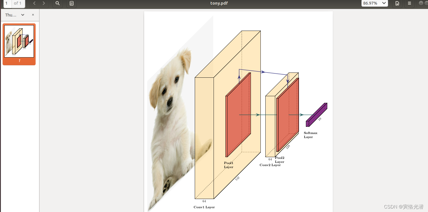
可以看到生成的可视化架构图，相比较于以前手工做图来说，真的大大提高了效率。更多详情可以去看具体源码。

github：PlotNeuralNet