孙玉龙版本的的pytorch实战浅析（本文章针对自己按照书本代码进行联系的浅析）

chap5：MLp（全连接层神经网络）

需要的数据（spambase.csv）的提取地址：链接：https://pan.baidu.com/s/1w182cRQEIExopdlyms-16g 
提取码：0113 
本文的数据是放在了spam=pd.read_csv("D:/jupyter/data/chap5/spambase.csv")，读者在做练习的时候需要到网盘去下载spambase.csv，并将放到自己定义的位置处，然后需要改spam读取数据的地址（本文的这个数据，第一行的已经做了改动，但是最后一列的标签列没做改动，不影响做练习）

import numpy as np
import pandas as pd
from sklearn.preprocessing import StandardScaler,MinMaxScaler
from sklearn.model_selection import train_test_split
from sklearn.metrics import accuracy_score,confusion_matrix,classification_report
from sklearn.manifold import TSNE


import torch
import torch.nn as nn
from torch.optim import SGD,Adam
import torch.utils.data as Data

import matplotlib.pyplot as plt
import seaborn as sns
import hiddenlayer as hl
from torchviz import make_dot

spam=pd.read_csv("D:/jupyter/data/chap5/spambase.csv")
pd.value_counts(spam.label) #读取csv对应的label列对应的0和1标签的个数,因为是二分类问题，这一列其实也就是我们预测的结果列（我们预测的结果就是0和1）
X=spam.iloc[:,0:57].values#将数据进行切分，将第0列到第56列的数据切分出来，采用.iloc，这个0到56列就是我们的输入，记得[0:57]就是我们对应的第0列到第56列
y=spam.label.values
X_train,X_test,y_train,y_test=train_test_split(X,y,test_size=0.25,random_state=123) #采用train_test_split进行对数据切分，测试集占用了25%，这是封装好的库
scale=MinMaxScaler(feature_range=(0,1))#将数据进行标准化
X_train_s=scale.fit_transform(X_train)#将标准化的数据进行拟合
X_test_s=scale.fit_transform(X_test)

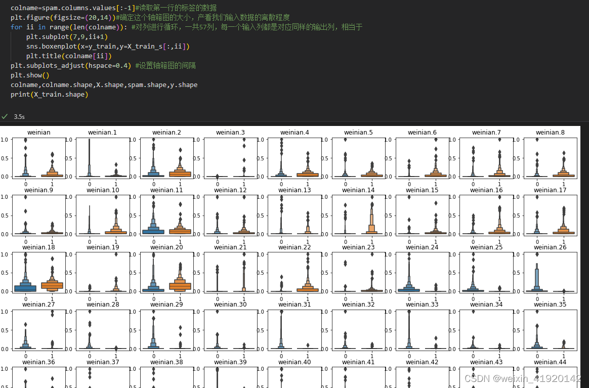
colname=spam.columns.values[:-1]#读取第一行的标签的数据
plt.figure(figsize=(20,14))#确定这个轴箱图的大小，产看我们输入数据的离散程度
for ii in range(len(colname)): #对列进行循环，一共57列，每一个输入列都是对应同样的输出列，相当于
    plt.subplot(7,9,ii+1)
    sns.boxenplot(x=y_train,y=X_train_s[:,ii])
    plt.title(colname[ii])
plt.subplots_adjust(hspace=0.4) #设置轴箱图的间隔
plt.show()
colname,colname.shape,X.shape,spam.shape,y.shape
print(X_train.shape)

class MLPclassifica(nn.Module): #定义了分类的神经网络结构，Linear的全连接层，会自动进行in_feature和out_feature的转置；神经我网络结构为两个全连接层和一个分类层，然后将前向传播的函数定义好
    def __init__(self):
        super(MLPclassifica,self).__init__()
        self.hidden1=nn.Sequential(
            nn.Linear(
                in_features=57,
                out_features=30,
                bias=True
            ),
            nn.ReLU()
        )
        self.hidden2=nn.Sequential(
            nn.Linear(
                in_features=30,
                out_features=10),
                nn.ReLU()
        )
        self.classifica=nn.Sequential(
            nn.Linear(10,2),
            nn.Sigmoid()
        )
    def forward (self,x):
            fc1=self.hidden1(x)
            fc2=self.hidden2(fc1)
            output=self.classifica(fc2)
            return fc1,fc2,output

#将数据进行转换为对应的tensor，这样pytorch才可以识别
X_train_nots=torch.from_numpy(X_train_s.astype(np.float32))
y_train_t=torch.from_numpy(y_train.astype(np.int64))
X_test_nots=torch.from_numpy(X_test_s.astype(np.float32))
y_test_t=torch.from_numpy(y_test.astype(np.int64))
X_train_nots.dtype,y_train_t.dtype,X_test_nots.dtype,y_test_t.dtype
mlpc=MLPclassifica() #定义了类，首先要有一个函数=这个类，然后才可以调用他的parameters
#a=list(mlpc.parameters()) #定义的函数先要有一个mlpc=这个函数，然后在调用.parameters(),这个.parameters()为对应的神经元网络内部的权重w和b
#a

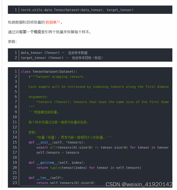
#定义一个载入的数据集，通过使用Dataloader可以对其进行小型的batch_size，这里注意这个batch_size最好可以整除数据样本数（例如有6400个样本，就可以使用batch_size为32或64等）
train_data_nots=Data.TensorDataset(X_train_nots,y_train_t)
train_nots_loader=Data.DataLoader(
    dataset=train_data_nots,
    batch_size=64,
    shuffle=True,#每次迭代都打乱顺序
    num_workers=1#同时开启几个进程，也就是其实和定义几个核数工作一样，就是可以提高运行的速度
)

optimizer=torch.optim.Adam(mlpc.parameters(),lr=0.01)
loss_func=nn.CrossEntropyLoss()

# 记录训练过程的指标
history1 = hl.History()
# 使用Canvas进行可视化
canvas1 = hl.Canvas()
print_step = 25

#pytorch其实很多地方都封装好了，内部的w和b的更新也自动定义好了，你只要给他传参就可以了，其他都可以不用定义，然后先梯度变0，然后计算损失函数，最后采用step（）进行梯度的更新即可
for epoch in range(15):
    for step,(b_x,b_y) in enumerate (train_nots_loader):
        _,_,output=mlpc(b_x) #这一步是得到了对应神经网络处理后得到的输出值
        train_loss=loss_func(output,b_y) #顺序必须为y_hat和y真实值
        optimizer.zero_grad()
        train_loss.backward()
        optimizer.step()
        niter=epoch*len(train_nots_loader)+step+1
        if niter % print_step==0:  #这里的output为预测的值，采用测试集的x作为输入，得到的对应的输出值
            _,_,output=mlpc(X_test_nots)
            _,pre_lab=torch.max(output,1) #0，1分类，10个输入，就会得到10*2的输出，一列为0的预测的10输出，一列为1标签对应的10个输出，.max（，1）找到每行对应的最大值的位置（这个最大值就是预测是0或者1，0那列的概率大则预测为0）
            test_accuracy=accuracy_score(y_test_t,pre_lab) #y_test的值为0或1，而pre_load的输出值也为0，1，正好进行比较他们之间的准确度；假如做二分类问题的y_test是单纯的标签，不是0-1标签，需要对y_test先进行转换。
            history1.log((niter,step), train_loss=train_loss, 
                         test_accuracy=test_accuracy)
            with canvas1:
                canvas1.draw_plot(history1["train_loss"])
                canvas1.draw_plot(history1["test_accuracy"])

_,_,output=mlpc(X_test_nots)#mlpc return了3个值，分别为fc1，fc2和output（最终的输出值），我们这里只需要一个最终的输出值，也就是y_hat
_,pre_lab=torch.max(output,1) #0，1分类，10个输入，就会得到10*2的输出，一列为0的预测的10输出，一列为1标签对应的10个输出，.max（，1）找到每行对应的最大值的位置（这个最大值就是预测是0或者1，0那列的概率大则预测为0）
test_accuracy=accuracy_score(y_test_t,pre_lab) #y_test的值为0或1，而pre_load的输出值也为0，1，正好进行比较他们之间的准确度；假如做二分类问题的y_test是单纯的标签，不是0-1标签，需要
print("test_accuracy:"+str(test_accuracy))

            

chap5-回归

 

 

 

 

 

## 导入本章所需要的模块
import numpy as np
import pandas as pd
from sklearn.preprocessing import StandardScaler
from sklearn.model_selection import train_test_split
from sklearn.metrics import mean_squared_error,mean_absolute_error
from sklearn.datasets import fetch_california_housing


import torch
import torch.nn as nn
import torch.nn.functional as F
from torch.optim import SGD
import torch.utils.data as Data

import matplotlib.pyplot as plt
import seaborn as sns
import hiddenlayer as hl
housdata = fetch_california_housing()
#pd.DataFrame（data(输入的数据)，columns为列的标签索引名（也就是标签），index为行的标签索引名
X_train,X_test,y_train,y_test=train_test_split(housdata.data,housdata.target,test_size=0.3,random_state=42)
scale=StandardScaler()
X_train_s=scale.fit_transform(X_train)
X_test_s=scale.transform(X_test)#测试集合不需要进行拟合
housdatadf=pd.DataFrame(data=X_train_s,columns=housdata.feature_names)#housdata.feature_names获取对应的列的标签
print(housdatadf.shape)
housdatadf["target"]=y_train #为这个housdatadf在添加一列，标签为target，数据为y_train，数据由原来的（14448，8）变为了（14448，9）
print(housdatadf.shape)
housdatadf["target"]=y_train #为这个housdatadf在添加一列，标签为target，数据为y_train，数据由原来的（14448，8）变为了（14448，9）
print(housdatadf.shape)
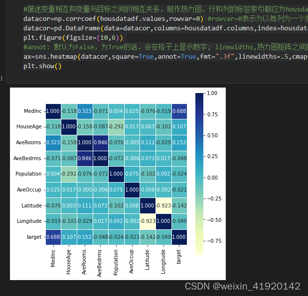
#描述变量相互和变量与目标之间的相互关系，制作热力图，行和列的标签索引都应为housdatadf.columns的标签名
datacor=np.corrcoef(housdatadf.values,rowvar=0) #rowvar=0表示为以每列为一个变量，当rowvar使用默认值或者rowvar=1时，以每一行为一个变量
datacor=pd.DataFrame(data=datacor,columns=housdatadf.columns,index=housdatadf.columns)
plt.figure(figsize=(10,6))
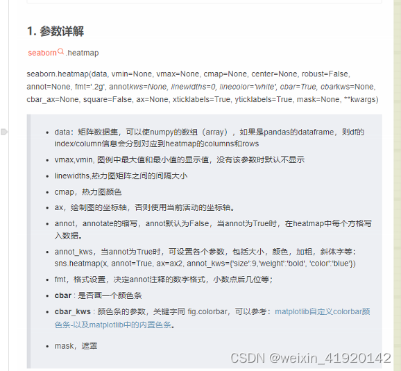
#annot: 默认为False，为True的话，会在格子上显示数字; linewidths,热力图矩阵之间的间隔大小;square:是否是正方形;cmap，热力图颜色;cbar_kws : 颜色条的参数
ax=sns.heatmap(datacor,square=True,annot=True,fmt=".3f",linewidths=.5,cmap="YlGnBu",cbar_kws={"fraction":0.46,"pad":0.03})
plt.show()
train_xt=torch.from_numpy(X_train_s.astype(np.float32))
train_yt=torch.from_numpy(y_train.astype(np.float32))
test_xt=torch.from_numpy(X_test_s.astype(np.float32))
test_yt=torch.from_numpy(y_test.astype(np.float32))
train_data=Data.TensorDataset(train_xt,train_yt)
test_data=Data.TensorDataset(test_xt,test_yt)
#载入数据，dataset= 载入的数据,batch_size为对应的批处理的大小
train_loader=Data.DataLoader(dataset=train_data,batch_size=64,shuffle=True,num_workers=1)
class MLPregression(nn.Module):
    def __init__(self):
        super(MLPregression,self).__init__()
        self.hidden1=nn.Linear(in_features=8,out_features=100,bias=True)
        self.hidden2=nn.Linear(100,100)
        self.hidden3=nn.Linear(100,50)
        self.predict=nn.Linear(50,1)
    def forward(self,x):
        x=F.relu(self.hidden1(x))
        x=F.relu(self.hidden2(x))
        x=F.relu(self.hidden3(x))
        output=self.predict(x)
        return output[:,0]

mlpreg=MLPregression()
proptimizer=torch.optim.SGD(mlpreg.parameters(),lr=0.01)
loss_func=nn.MSELoss()#使用了均方根误差损失函数的方法
train_loss_all=[]#先定义每一此epoch的总损失值为train_loss_all,定义为矩阵形式，然后后面就可以用append了
for epoch in range(30):
    train_loss=0
    train_num=0
    for step,(b_x,b_y) in enumerate (train_loader):
         output=mlpreg(b_x)
         loss=loss_func(output,b_y) #求解的是这个批次（b_x.size(0)）的平均损失值
         optimizer.zero_grad()
         loss.backward()
         optimizer.step()
         train_loss +=loss.item()*b_x.size(0) #item()就是将值转化为数值,这里loss得出的损失值是单个的，必须*b_x.size(0),相当于有这个批次有64个，损失值=平均损失值*64（64就是b_x.size(0)）
         train_num+=b_x.size(0)#这里为样本数，也就是上一个案例用什么epoch*len（train_loader)+step+1这种类似
    train_loss_all.append(train_loss/train_num)
int(mlpreg)
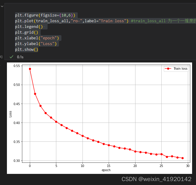
plt.figure(figsize=(10,6))
plt.plot(train_loss_all,"ro-",label="Train loss") #train_loss_all 为一个一维度的数据，相当于画图的y，plt会自动补齐x，x就是对应1，2，3这样的东西
plt.legend() 
plt.grid()
plt.xlabel("epoch")
plt.ylabel("Loss")
plt.show()
## 可视化在测试集上真实值和预测值的差异
index = np.argsort(y_test) #将y_test的元素按照大小进行排序
print(index.shape)
plt.figure(figsize=(12,5)) 
plt.plot(np.arange(len(y_test)),y_test[index],"r",label = "Original Y") #将原始的y_test画出来，横轴为大小的序号，用np.arange(len(y_test))来产生1-6192（index的维度）的数
plt.scatter(np.arange(len(pre_y)),pre_y[index],s = 3,c = "b",label = "Prediction") #用散点图画出对应的预测的y_hat的散点图（因为y_hat为离散数据，所以需要用散点图）
plt.legend(loc = "upper left")
plt.grid()
plt.xlabel("Index")
plt.ylabel("Y")
plt.show()