VAE详解

1. 背景知识

1.1 ELBo

1.1.1 为什么引入隐变量 $z$ ?

因为我们在现实世界看到的物体可能也产生于高层级的表示，这样的表示或许概括了颜色、大小、形状等的抽象属性。

1.1.2 如何推导ELBo (Evidence Lower Bound)？

无条件的生成模型学习的是如何建模真实分布 $p\left(x\right)$ ，所以有：

$$\begin{array}{rl}\log \underset{\text{e}vidence}{\underbrace{p\left(x\right)}}& =\log p\left(x\right)\int \underset{\text{approximate posterior}}{\underbrace{q_{\varphi }\left(z|x\right)}}dz\\ & =\int q_{\varphi }\left(z|x\right)\left(\log p\left(x\right)\right)dz\\ & ={\mathbb{E}}_{q_{\varphi }\left(z|x\right)}\left[\log p\left(x\right)\right]\\ & ={\mathbb{E}}_{q_{\varphi }\left(z|x\right)}\left[\log \frac{p\left(x,z\right)}{p\left(z|x\right)}\right]\\ & ={\mathbb{E}}_{q_{\varphi }\left(z|x\right)}\left[\log \frac{p\left(x,z\right)q_{\varphi }\left(z|x\right)}{p\left(z|x\right)q_{\varphi }\left(z|x\right)}\right]\\ & ={\mathbb{E}}_{q_{\varphi }\left(z|x\right)}\left[\log \frac{p\left(x,z\right)}{q_{\varphi }\left(z|x\right)}\right]+{\mathbb{E}}_{q_{\varphi }\left(z|x\right)}\left[\log \frac{q_{\varphi }\left(z|x\right)}{p\left(z|x\right)}\right]\\ & =\underset{\text{ELBo}}{\underbrace{{\mathbb{E}}_{q_{\varphi }\left(z|x\right)}\left[\log \frac{p\left(x,z\right)}{q_{\varphi }\left(z|x\right)}\right]}}+\underset{\ge 0}{\underbrace{D_{KL}\left(\underset{\text{approximate posterior}}{\underbrace{q_{\varphi }\left(z|x\right)}}\Vert \underset{\text{true posterior}}{\underbrace{p\left(z|x\right)}}\right)}}\\ & \ge \underset{\text{ELBo}}{\underbrace{{\mathbb{E}}_{q_{\varphi }\left(z|x\right)}\left[\log \frac{p\left(x,z\right)}{q_{\varphi }\left(z|x\right)}\right]}}\end{array}$$

1.1.3 为什么要去最大化ELBo?

原因1：因为我们想要模型学习近似后验 $q_{\varphi }\left(z|x\right)$ 无限接近真实后验 $p\left(z|x\right)$，但是无法直接去求公式 (7) 中的 $D_{KL}$ 项：

$$\begin{array}{r}\underset{\varphi }{\min }\underset{\text{untractable}}{\underbrace{D_{KL}\left(\underset{\text{Encoder is learnable}}{\underbrace{\underset{\text{approximate posterior}}{\underbrace{q_{\varphi }\left(z|x\right)}}}}\Vert \underset{\text{unknow}}{\underbrace{\underset{\text{true posterior}}{\underbrace{p\left(z|x\right)}}}}\right)}}\end{array}$$

原因2：对于任意的样本$x_i\sim p\left(x\right)$，$p\left(x_i\right)$是个常数，那么通过${\max }_{\varphi }\text{ELBo}$等价于${\min }_{\varphi }{D}_{KL}$
$$\begin{array}{rl}\because \log \underset{\text{c}onstant}{\underbrace{p\left(x_i\right)}}& =\underset{\text{ELBo}}{\underbrace{{\mathbb{E}}_{q_{\varphi }\left(z|x_i\right)}\left[\log \frac{p\left(x_i,z\right)}{q_{\varphi }\left(z|x_i\right)}\right]}}+\underset{\ge 0}{\underbrace{D_{KL}\left(\underset{\text{approximate posterior}}{\underbrace{q_{\varphi }\left(z|x_i\right)}}\Vert \underset{\text{true posterior}}{\underbrace{p\left(z|x_i\right)}}\right)}}\\ \underset{\varphi }{\min }{D}_{KL}& ⟺\underset{\varphi }{\max }\text{ELBo}\end{array}$$

2. VAE (Variational Autoencoder)

2.1 为什么Variational?

因为我们优化的 $q_{\varphi }\left(z|x\right)$ 服从某一分布族，该分布族被 $\varphi$ 参数化，这就是 Variational 的来源。

2.2 为什么Autoencoder？

因为模型会像AE (Autoencoder) 模型一样压缩数据维度，提取数据中的有效信息。

2.3 VAE的优化目标是什么？

$$\begin{array}{rl}& \underset{\varphi }{\max }\underset{\text{ELBo}}{\underbrace{{\mathbb{E}}_{q_{\varphi }\left(z|x\right)}\left[\log \frac{p\left(x,z\right)}{q_{\varphi }\left(z|x\right)}\right]}}\\ & =\underset{\varphi ,\theta }{\max }{\mathbb{E}}_{q_{\varphi }\left(z|x\right)}\left[\log \frac{p_{\theta }\left(x|z\right)p\left(z\right)}{q_{\varphi }\left(z|x\right)}\right]\\ & =\underset{\varphi ,\theta }{\max }{\mathbb{E}}_{q_{\varphi }\left(z|x\right)}\left[\log p_{\theta }\left(x|z\right)\right]+{\mathbb{E}}_{q_{\varphi }\left(z|x\right)}\left[\frac{p\left(z\right)}{q_{\varphi }\left(z|x\right)}\right]\\ & =\underset{\varphi ,\theta }{\max }\underset{\text{resconstraction term}}{\underbrace{{\mathbb{E}}_{q_{\varphi }\left(z|x\right)}\left[\log \underset{\text{Decoder}}{\underbrace{p_{\theta }\left(x|z\right)}}\right]}}-\underset{\text{prior matching term}}{\underbrace{D_{KL}\left(\underset{\text{Encoder}}{\underbrace{q_{\varphi }\left(z|x\right)}}\Vert \underset{\text{prior}}{\underbrace{p\left(z\right)}}\right)}}\\ & \stackrel{\text{Monte Carlo Estimate}}{\approx }\underset{\varphi ,\theta }{\max }\sum _{l=1}^L\log p_{\theta }\left(x|z^l\right)-D_{KL}\left(\underset{\sim N\left(\mu ,{\sigma }^2\right)}{\underbrace{q_{\varphi }\left(z|x\right)}}\Vert \underset{\sim N\left(0,1\right)}{\underbrace{p\left(z\right)}}\right)\\ & =\underset{\varphi ,\theta }{\max }\sum _{l=1}^L\log p_{\theta }\left(x|z^l\right)-\frac{1}{2}\left(-\log {\sigma }^2+{\mu }^2+{\sigma }^2-1\right)\end{array}$$

由等式 (15) (16) 可知，优化目标主要包括了两项：重构项 (reconstruction term) 迫使模型的解码器 (Decoder) 学习由隐变量 $z$ 恢复原始样本的能力；先验匹配项 (prior matching term) 迫使模型的编码器 (Encoder) 学习将原始样本转换到先验分布 (标准正态分布) 的能力。

2.4 VAE模型架构

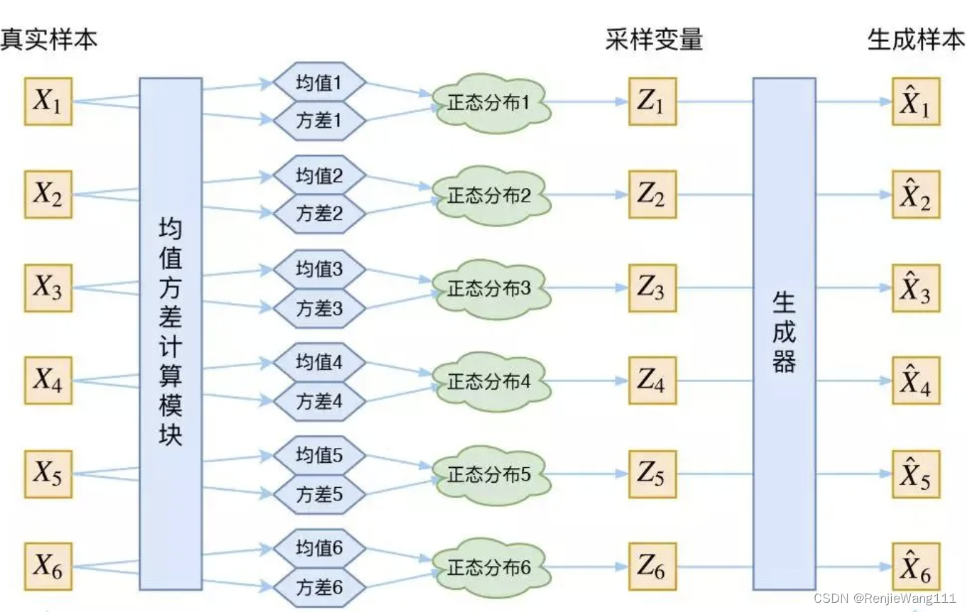
3. VAE的训练

训练过程将批量的图片送入模型中，每张图片由 Encoder 产生 $\mu$ 和 $\sigma$，进而生成服从 $N\left(\mu ,{\sigma }^2\right)$ 的隐变量 $z$，最后经过 Decoder 生成图片，整体流程如下：

$$\underset{x\sim p\left(x\right)}{\underbrace{x}}\to \underset{q_{\varphi }\left(z|x\right)}{\underbrace{\text{Encoder}}}\to \mu ,\sigma \to \underset{\text{reparameterization trick}}{\underbrace{\underset{z=\mu +\sigma \odot ϵ,\text{with }ϵ\sim N\left(0,I\right)}{\underbrace{z\sim \mathbf{N}\left(\mu ,{\sigma }^2\right)}}}}\to \underset{p_{\theta }\left(x|z\right)}{\underbrace{\text{Decoder}}}\to \hat{x}$$

其中，训练过程中会采用重参数化技巧 (reparameterization trick) 使得整个过程可导，因为这样 $\mu$ 和 $\sigma$ 变成可导的参数，变化的 $ϵ$ 被看作不用求导的常数，不被算在梯度图中。

4. VAE的推理

推理只需要从标准正态分布中采样隐变量 $z$ 即可以生成新的样本，因为 VAE 目标函数中的先验匹配项迫使 $z$ 逐渐逼近标准正态分布，整体流程如下：

$$\underset{\mathbf{z}\sim \mathbf{N}\left(0,\mathbf{I}\right)}{\underbrace{z}}\to \underset{p_{\theta }\left(x|z\right)}{\underbrace{\text{Decoder}}}\to \underset{\text{new sample}}{\underbrace{\hat{x}}}$$