Matlab读取NetCDF文件及绘图

Matlab读取NetCDF文件及绘图

1. 读取文件

ncload('gls_avg_output.nc');%读取整个文件
ncload('gls_avg_output.nc','var1','var2');%读取文件中的某几个变量

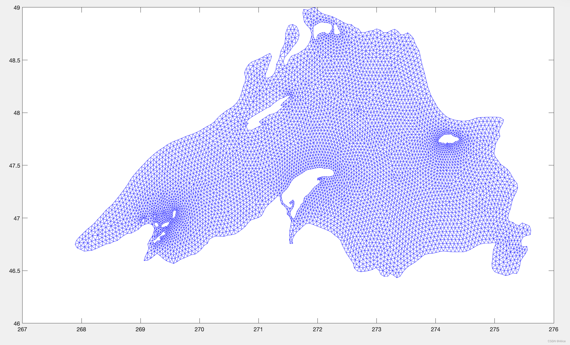
2. 绘制网格图

%m=size(nv,1);
%n=size(nv,2);
[m,n]=size(nv);
for i=1:n
    a1(i)=nv(1,i);%nv means nodes surrounding element
    a2(i)=nv(2,i);
    a3(i)=nv(3,i);

    b1(:,i)=[a1(i) a2(i) a3(i) a1(i)];   
end
plot (lon(b1), lat(b1),'color','b')

• 几个概念：
• node：表示三角形的顶点
• center：表示三角形的中心
• element/cell：表示三角形
• 所以center的个数=element的个数，且约等于node个数的2倍
• layer：纵向有厚度的层
• level：layer的上下边界
• temperature，zeta和salinity记录在node上，速度u，v记录在center，速度w记录在level上。
  

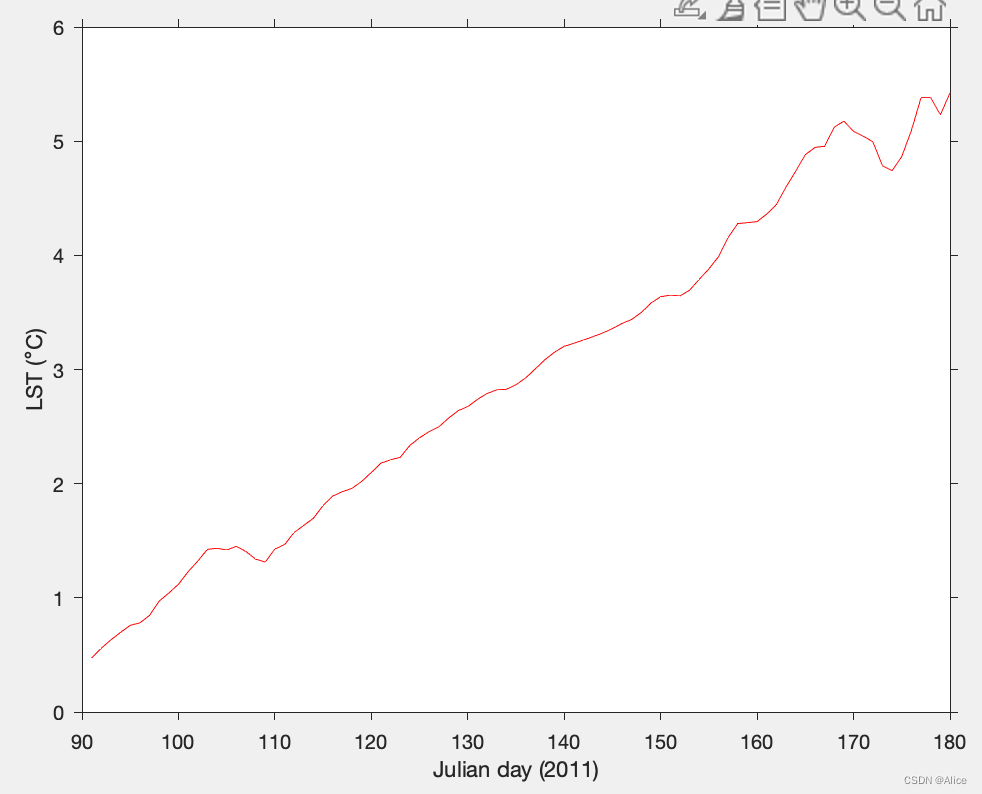
3. 计算并绘制平均水面温度（avg lake surface temperature）

clear lst
lst=squeeze(temp(:,1,:));%去掉多余的维度
[nt,nn]=size(lst)
for t=1:nt
    lst_avg(t)=sum(lst(t,:).*art1')./sum(art1);%按照网格面积求温度的加权平均
end

figure(101);clf;hold on;box on;%clf清空图窗
    set(gca,'tickdir','out');%坐标轴刻度向外
    plot([1:length(lst_avg)]+90,lst_avg,'r');
    xlabel(['Julian day (' num2str(yr) ')']);
    ylabel('LST (\circC)');
    text(-92,5.5,['Lake-wide aerage LST']);
    
saveas(gcf,['fig_lake_wide_avg_lst_' num2str(yr) '.png'],'png');  

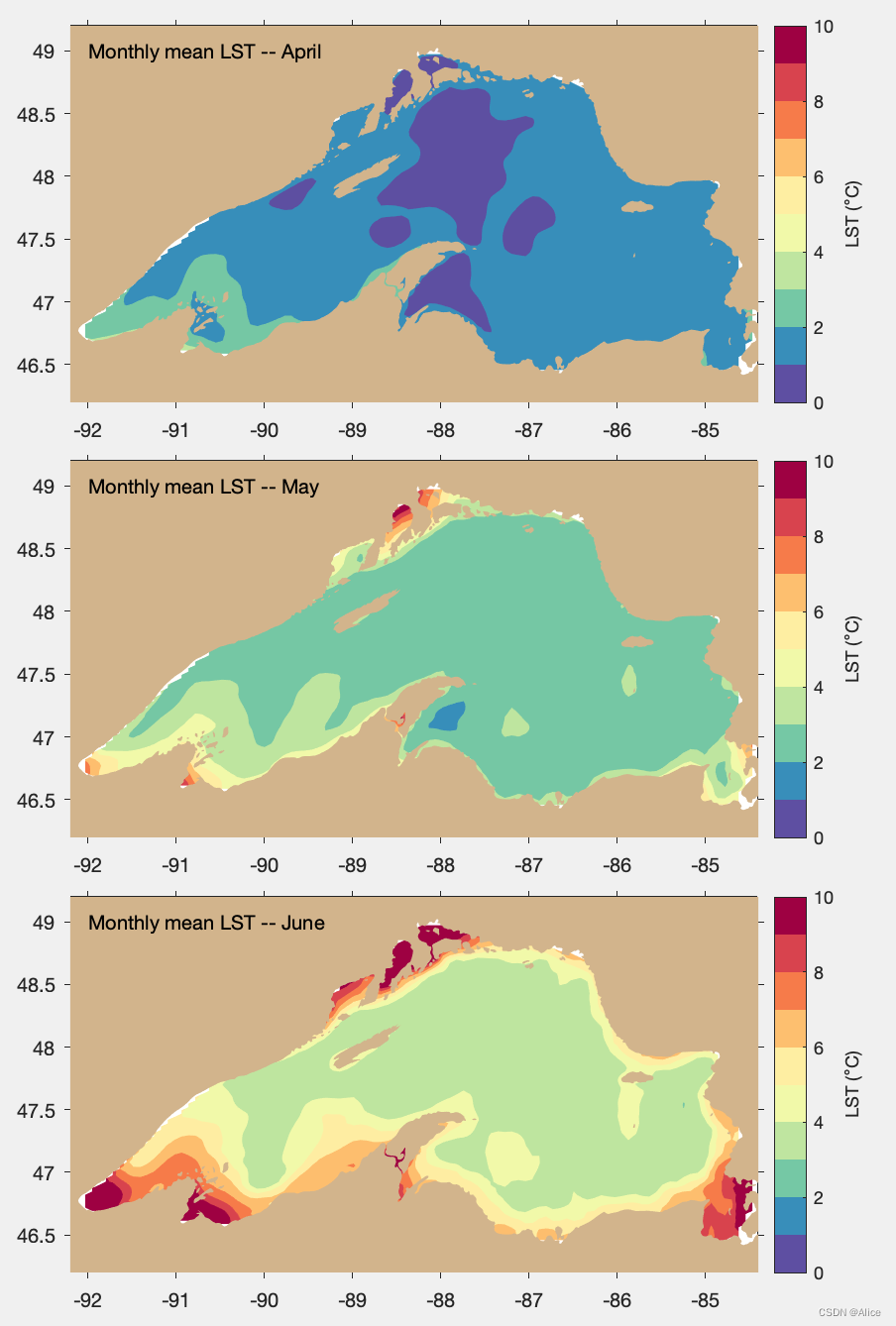
4. 绘制月平均湖表面温度在湖表面的分布（contour）

clear lst_mm
size(lst)
lst_mm=mean_by_segments(lst,[0:30:90],1);%自定义函数，可以按月（28天/30天/31天）取平均
size(lst_mm)

cmin=0;cinc=1;cmax=10;%colorbar的上下限及间隔
ncc=round([cmax-cmin]/cinc);%colorbar所需颜色数量
ccmap=flipud(spectral(ncc));%颠倒矩阵，即使冷色表示低温，暖色表示高温
%ccmap=parula(ncc);

figure(201);clf;hold on;set_portrait;

    hh1=subplot(3,1,1);cla;hold on;box on;
    hh1_pp=get(hh1,'position');%将hh1中的position赋值给hh1-pp
    set(hh1,'position',hh1_pp+[0.1 0 -0.2 0]);%设置图片位置
    set(gca,'tickdir','out');
    scattercontourf(xlon,xlat,lst_mm(1,:)',[cmin:cinc:cmax]);%通过散点画contour图（自定义的函数）
    caxis([cmin cmax]);%设置colorbar的上下限
    colormap(hh1,ccmap);%设置colormap的颜色
    plot_fvcom_obc(map,[210 180 140]/255);%绘制陆地
    axis([-92.2 -84.4 46.2 49.2]);%设置坐标
    lcb=colorbar('location','eastoutside');%设置colorbar所在位置
    ylabel(lcb,'LST (\circC)');
    text(-92,49,'Monthly mean LST -- April');
    % colormap(ax(1), ccmap)


    %
    hh2=subplot(3,1,2);cla;hold on;box on;
    hh2_pp=get(hh2,'position');
    set(hh2,'position',hh2_pp+[0.1 0.05 -0.2 0]);%set figure 
    set(gca,'tickdir','out');
    scattercontourf(xlon,xlat,lst_mm(2,:)',[cmin:cinc:cmax]);
    caxis([cmin cmax]);
    colormap(hh2,ccmap);
    plot_fvcom_obc(map,[210 180 140]/255);
    axis([-92.2 -84.4 46.2 49.2]);
    lcb=colorbar('location','eastoutside');
    ylabel(lcb,'LST (\circC)');
    text(-92,49,'Monthly mean LST -- May');

   %
    hh3=subplot(3,1,3);cla;hold on;box on;
    hh3_pp=get(hh3,'position');
    set(hh3,'position',hh3_pp+[0.1 0.1 -0.2 0]);
    set(gca,'tickdir','out');
    scattercontourf(xlon,xlat,lst_mm(3,:)',[cmin:cinc:cmax]);
    caxis([cmin cmax]);
    colormap(hh3,ccmap);
    plot_fvcom_obc(map,[210 180 140]/255);
    axis([-92.2 -84.4 46.2 49.2]);
    lcb=colorbar('location','eastoutside');
    ylabel(lcb,'LST (\circC)');
    text(-92,49,'Monthly mean LST -- June');

    hh1.Colormap=ccmap;
    hh2.Colormap=ccmap;
    hh3.Colormap=ccmap;
    
 saveas(gcf,['fig_lake_lst_monthly_mean_pattern_' num2str(yr) '.png'],'png');  

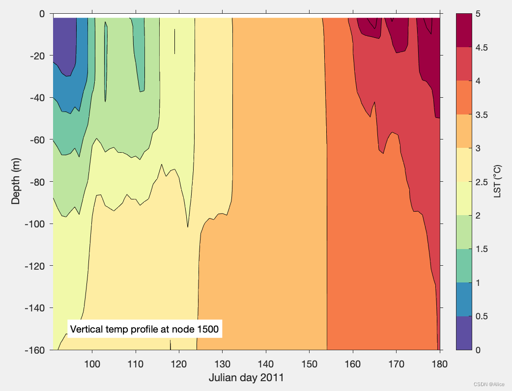
5. 绘制水平上某点处的温度在水深上的分布随时间的变化

pp=1500%选取某一点

xx=[1:nt]+90;
yy=h(pp).*siglay(:,pp);%每一层的水深
dd=squeeze(temp(:,:,pp));

cmin=0;cinc=0.5;cmax=5;
ncc=round([cmax-cmin]/cinc);
ccmap=flipud(spectral(ncc));

figure(301);clf;hold on;box on;
    set(gca,'tickdir','out');
    contourf(xx,yy,dd',[cmin:cinc:cmax]);
    caxis([cmin cmax]);
    colormap(ccmap);
    plot_fvcom_obc(map,[210 180 140]/255);
    axis([91 180 -160 0]);
    lcb=colorbar('location','eastoutside');
    ylabel(lcb,'LST (\circC)');
    text(95,-150,['Vertical temp profile at node ' num2str(pp)],'background','w');
    xlabel(['Julian day ' num2str(yr)]);
    ylabel(['Depth (m)'])
    %