Lake Michigan Data assimilation

最新推荐文章于 2024-07-19 20:47:39 发布

Alice

最新推荐文章于 2024-07-19 20:47:39 发布

阅读量1.5k

点赞数 36

文章标签：前端 javascript chrome

本文链接：https://blog.csdn.net/weixin_42222933/article/details/139638521

版权

1. Run without DA to get the spatial SST to calculate error correlation, based on which weight can be generated.

Take year 2009 as an example. I have set up the folder, and the path is: /pexue6/chuyan/lake_michigan/year_2009/no_da


[czhao4@compute-0-201 no_da]$ cd /pexue6/chuyan/lake_michigan/year_2009/no_da
# This folder should contain:
[czhao4@compute-0-201 no_da]$ ls
fvcom  fvcom.sh  glmHR_run.nml  input  output  run.sh
# "fvcom" does not need any modify
# "fvcom.sh" can be generated by "qgenscript", or simply modify the CUSTOM_PROGRAM_PATH to the present path. If you use qgenscript, I usually use 64 CPUs.
[czhao4@compute-0-201 no_da]$ vi fvcom.sh 
CUSTOM_PROGRAM_PATH="/pexue6/chuyan/lake_michigan/year_2009/no_da"
# Modify all the "year" in the namelist "glmHR_run.nml"
[czhao4@compute-0-201 no_da]$ vi glmHR_run.nml
START_DATE      = '2009-01-01 00:00:00'
END_DATE        = '2010-01-01 00:00:00'

RST_FIRST_OUT    = '2009-12-31 00:00:00'

NC_FIRST_OUT    = '2009-01-01 00:00:00'

NCSF_FIRST_OUT = '2009-01-01 00:00:00'

NCAV_FIRST_OUT       = '2009-01-01 00:00:00'

WIND_FILE    = 'glmHR_forcing_marobs_2009.nc'

AIRPRESSURE_FILE  = 'glmHR_forcing_marobs_2009.nc'

HEATING_CALCULATE_FILE  = 'glmHR_forcing_marobs_2009.nc'
# set up input folder
[czhao4@compute-0-201 no_da]$ cd input
# link from xinyu's folder. The path for the other year please see below.
[czhao4@compute-0-201 input]$ ln -s /pexue5/xinyuy/year_2009/input/* --exclude=glmHR_sst_grid_test_weight_2009.nc ./
[czhao4@compute-0-201 input]$ ls
glmHR_cor.dat  glmHR_forcing_marobs_2009.nc  glmHR_obc.dat    glmHR_spg.dat
glmHR_dep.dat  glmHR_grd.dat                 glmHR_sigma.dat
# link restart file from last year
[czhao4@compute-0-201 input]$ ln -s /pexue6/chuyan/lake_michigan/year_2008/no_da/output/glmHR_restart_0001.nc ./
[czhao4@compute-0-201 input]$ ls
glmHR_cor.dat  glmHR_forcing_marobs_2009.nc  glmHR_obc.dat          glmHR_sigma.dat
glmHR_dep.dat  glmHR_grd.dat                 glmHR_restart_0001.nc  glmHR_spg.dat
# The setup is all done now! 
[czhao4@compute-0-201 input]$ cd ../
[czhao4@compute-0-201 no_da]$ qsub fvcom.sh

** you need to change “output” to “input” to find the forcing files
Lake Michigan:
/pexue4/xinyuy/DA_run_sst_assim_adjust/year_1995/output

/pexue4/xinyuy/DA_run_sst_assim_adjust/year_1996/output

/pexue5/xinyuy/year_1997/output/

/pexue5/xinyuy/year_1998/output/
/pexue5/xinyuy/year_1999/output/
/pexue5/xinyuy/year_2000/output/
/pexue5/xinyuy/year_2001/output/
/pexue5/xinyuy/year_2002/output/
/pexue5/xinyuy/year_2003/output/
/pexue5/xinyuy/year_2004/output/
/pexue5/xinyuy/year_2005/output/
/pexue5/xinyuy/year_2006/output/
/pexue5/xinyuy/year_2007/output/
/pexue5/xinyuy/year_2008/output/
/pexue5/xinyuy/year_2009/output/
/pexue4/xinyuy/DA_run_sst_assim_adjust/year_2010/output/

model for 2011 has two parts, since the model blew up at 10/19
part1: /pexue6/xinyuy/DA_new_run_2010-2020/2011_output/output/
part2: /pexue5/xinyuy/year_2011/output

/pexue6/xinyuy/DA_new_run_2010-2020/2012_output/output/
/pexue6/xinyuy/DA_new_run_2010-2020/2013_output/output/
/pexue6/xinyuy/DA_new_run_2010-2020/2014_output/output/
/pexue6/xinyuy/DA_new_run_2010-2020/2015_output/output/
/pexue4/xinyuy/DA_run_sst_assim_adjust/year_2016_new/output/
/pexue4/xinyuy/DA_run_sst_assim_adjust/year_2017/output_rerun

/pexue4/xinyuy/DA_run_sst_assim_adjust/year_2018_hrrr/output/

/pexue4/xinyuy/DA_run_sst_assim_adjust/year_2019_hrrr/output/

/pexue4/xinyuy/DA_run_sst_assim_adjust/year_2020_hrrr/output/

2. Run with DA

Generate weight files by MATLAB
(1) download spatial SST.

[czhao4@compute-0-201 no_da]$ cd output/
[czhao4@compute-0-201 output]$ ls
glm_lst.sh  glm_vert_temp.sh
[czhao4@compute-0-201 output]$ vi glm_lst.sh 
for i in {1..366} # change 366 to 367 if it's leap year
do
printf -v nn "%04d" ${i}
xtmp="ncks -C -v lon,lat,h,art1,temp,Times -F -d siglay,1 glmHR_${nn}.nc tmp_${nn}.nc"
echo ${xtmp}
eval ${xtmp}
done
#
xtmp="ncrcat tmp_????.nc glm_lst_2009_LowRes.nc" # 2009
echo ${xtmp}
eval ${xtmp}
rm -f tmp_????.nc

[czhao4@compute-0-201 output]$ source glm_lst.sh

Then download the generated file “glm_lst_2009_LowRes.nc” to /year_2009/no_da on your computer.
(2) Generate weight files
I uploaded all the Matlab code in this Google Drive link, you can find year_2009 here as an example. https://drive.google.com/drive/folders/1RZqZrWJtKL8FBhbu3AUOvisdiZwwnf7i?usp=sharing

Go to /year_2009/weight/linux_file, move “weight_2003.nc” to /year_2009/weight, and rename it to “weight_2009.nc”. And clear the folder “linux_file”, we need to generate new files for year 2009 later.
For the leap year, you need to copy the weight_???.nc file from a leap year, because the length of the variables are different.
Go to /year_2009/weight, delete “gler_lm_temp_mooring_2009.mat”. We need to generate 2009 mooring data. Open “merge_obs_mooring.m”, modify “year” to 2009, and run.
You will need mooring data in the following link. https://drive.google.com/drive/folders/1YXIALwDnZoSoA0EWOsmOMQFkmSwdfgAs?usp=sharing
Open “create_sst_weight_nc.m”, modify year and day, and the obs data path, and then run. A new file will be generated in the /year_2009/weight/linux_file, you can check if the “Times” in the new file is correct.
You will need GLSEA sst data here. If you don’t have them on your computer, please find the following link.
https://drive.google.com/drive/folders/1wAAmT84wV7wR4BQn-fH5vGq9Ev_RrFM_?usp=sharing
Open “create_all_obs_ts_xy.m”, modify year, and the obs data path, and then run. A new file will be generated in the /year_2009/weight/linux_file.
Open “create_all_obs_ts_dat.m”, modify year and day, and the obs data path, and then run. A new file will be generated in the /year_2009/weight/linux_file.
Open “create_weight_control_dat.m”, modify year and day, and the obs data path, and then run. A new file will be generated in the /year_2009/weight/linux_file.
Check /year_2009/weight/linux_file, there should be 4 files in there:

(3) Set up the DA run
Upload all the 4 files to the input folder of DA run “/year_2009/da/input”
Link the forcing and restart files to the input folder, which are same with no_da run.
Then, the input folder should contain the following files:

[czhao4@compute-0-201 input]$ ls ../../../year_2001/da/input/
all_obs_ts.dat  glmHR_dep.dat                 glmHR_obc.dat          glmHR_spg.dat
all_obs_ts.xy   glmHR_forcing_marobs_2001.nc  glmHR_restart_0001.nc  weight_2001.nc
glmHR_cor.dat   glmHR_grd.dat                 glmHR_sigma.dat        weight_control.dat

Modify “fvcom.sh” and “glmHR_run.nml”, same with no_da run. But, please notice that the namelist of da run is different from no_da run. So DO NOT copy it from no_da run.
Modify “only_DA.nml” .

[czhao4@compute-0-201 da]$ vi only_DA.nml 
SSTGRD_ASSIM_FILE       = weight_2009.nc

The setup is all done!

[czhao4@compute-0-201 da]$ qsub fvcom.sh

3. Plot the results

All the mentioned Matlab code can be found in the google drive.
https://drive.google.com/drive/folders/1n4PHZfA8l49GN8Yym6b8pNcKlFM1atO1?usp=sharing

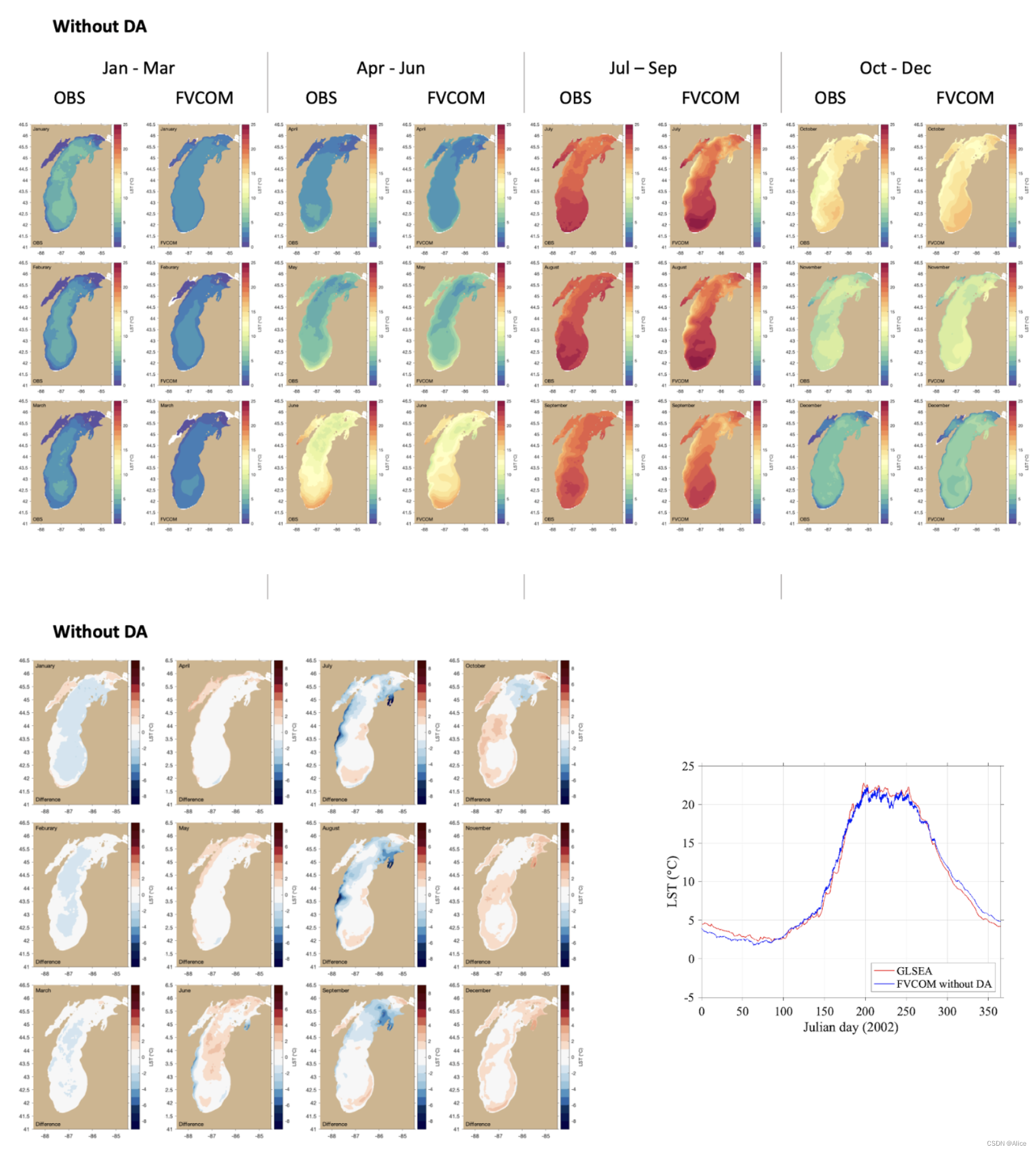
For sst, we need to plot lake-averaged sst and monthly spatial sst.

All the variables you need to modify are year, day and some observation data paths. Here are the plots you should get.
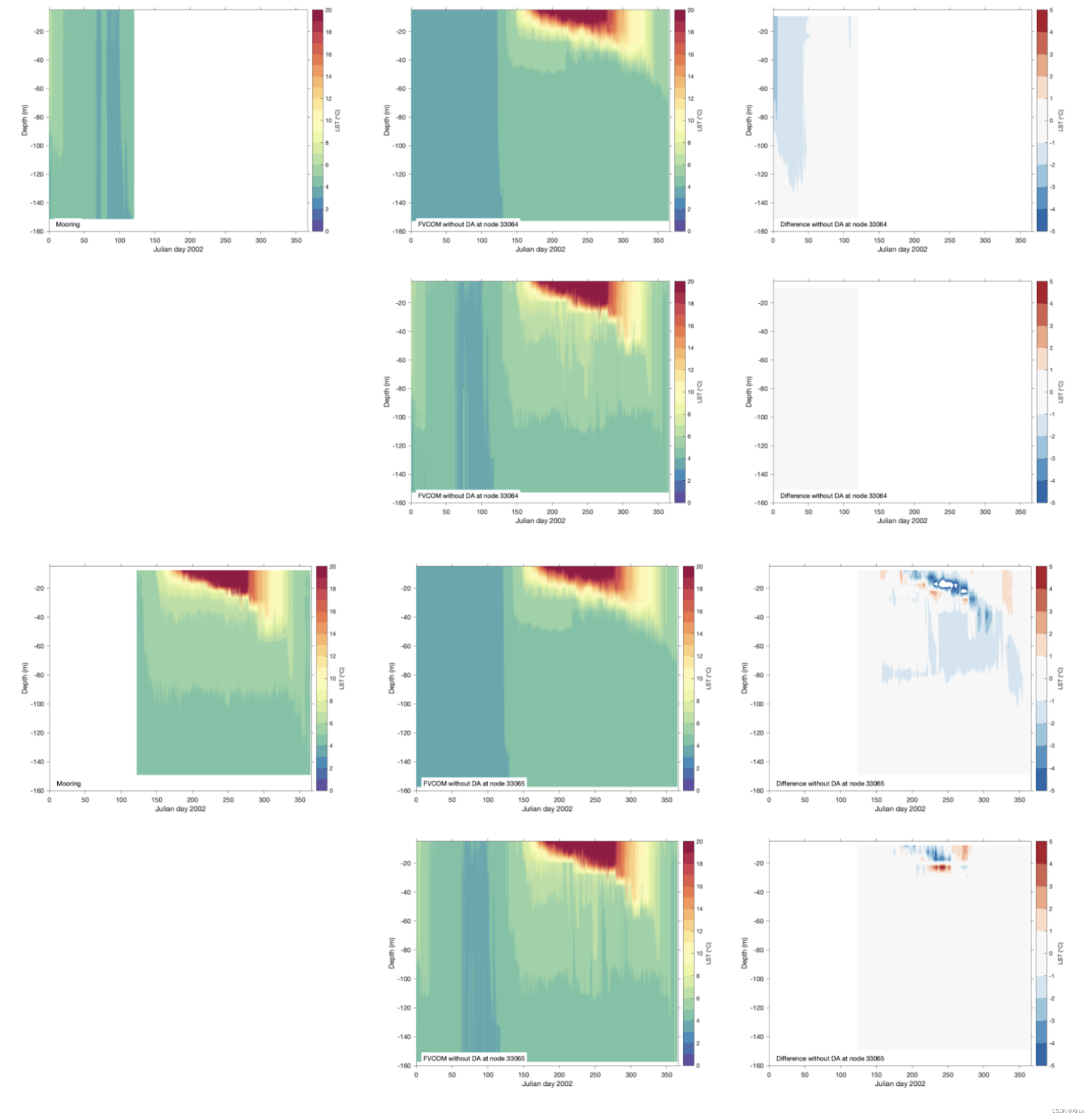
For thermal structure, we use: plot_vertical_temp.m or plot_vertical_temp_???.m, which depends if more than one mooring are available for the year.
You can check how many moorings are available by evaluate the first 56 lines of “plot_vertical_temp.m”. And then check the variable “pos_mod”. It shows the corresponding node of the mooring locations.
After you get the node number, go to HPC path: “year_2009/no_da/output/”

[czhao4@compute-0-201 da]$ cd year_2009/no_da/output/
[czhao4@compute-0-201 output]$ ls
glm_lst.sh  glm_vert_temp.sh
[czhao4@compute-0-201 output]$ vi glm_vert_temp.sh 

for i in {1..366} # change 366 to 367 if it's leap year
do
printf -v nn "%04d" ${i}
xtmp="ncks -C -v h,art1,temp,siglay,Times -F -d node,33312 glmHR_${nn}.nc tmp_${nn}.nc" # change 33312 to target node
echo ${xtmp}
eval ${xtmp}
done
#
xtmp="ncrcat tmp_????.nc glm_ver_temp_2000_LowRes_33312.nc" # change 33312 to target node
echo ${xtmp}
eval ${xtmp}
rm -f tmp_????.nc

[czhao4@compute-0-201 output]$ source glm_vert_temp.sh

Download the results and use plot_vertical_temp.m (can generate 2 nodes) or plot_vertical_temp_???.m (can generate only one node) to plot. Here are the plots you should get.
** Please note that sometimes the depths in the mooring observation are not increasing monotonously, that’s why lines 33- 39 exist. If they are monotonously, just turn them off.

tmp1=depth_obs(1).depth(1);
depth_obs(1).depth(1)=depth_obs(1).depth(2);
depth_obs(1).depth(2)=tmp1;

tmp2=temp_obs(1).temp(1);
temp_obs(1).depth(1)=temp_obs(1).temp(2);
temp_obs(1).depth(2)=tmp2;