李宏毅2020机器学习作业2——Classification

---

开始之前声明：本文参考了李宏毅机器学习作业说明（需翻墙），基本上是将代码复现了一遍，说明中用的是google colab（由谷歌提供的免费的云平台），我用的是Jupyter Notebook

---

本文用到的资料在百度网盘自取点击下载，提取码：zdth。请将所需资料下载解压，确保资料中有6个文件，并保存到自己的目录当中。

---

【博主的环境：Anaconda3+Jupyter Notebook，python3.6.8】

---

作业要求：根据收集来的资料，判断每个人其年收入是否高于50000美元，用Logistic regression和Generative model两种方法来实现

---

1.Logistic regression

---

现在开始跟着我一步步copy~~
开始之前导入需要用到的库：

• numpy:Python的一个扩展程序库，支持大量的维度数组与矩阵运算
• matplotlib：一个强大的绘图工具库

没有库的请自行安装（Jupyter Notebook安装方法：进入自己的环境，conda install 库名字 即可）

import numpy as np
#确保跟博主生成相同的随机数
np.random.seed(0)

添加路径

#添加文件路径
X_train_fpath = 'E:/jupyter/data/hw2/data/X_train'
Y_train_fpath = 'E:/jupyter/data/hw2/data/Y_train'
X_test_fpath = 'E:/jupyter/data/hw2/data/X_test'
output_fpath = 'E:/jupyter/work2/output_{}.csv'	#用于测试集的预测输出

加载数据,我们直接导入已经处理好的数据X_train,Y_train,X_test

#加载数据
with open(X_train_fpath) as f:
    next(f)
    X_train = np.array([line.strip('\n').split(',')[1:] for line in f], dtype = float)
with open(Y_train_fpath) as f:
    next(f)
    Y_train = np.array([line.strip('\n').split(',')[1] for line in f], dtype = float)
with open(X_test_fpath) as f:
    next(f)
    X_test = np.array([line.strip('\n').split(',')[1:] for line in f], dtype = float)

如果你想查看train数据是什么样的，可以用Notepad++打开查看，excel打开会出现乱码

然后我们编写一个_normalize()函数对数据进行预处理：归一化，即每个数据特征的均值和标准差进行归一化

#归一化
def _normalize(X, train = True, specified_column = None, X_mean = None, X_std = None):
    # This function normalizes specific columns of X.
    # The mean and standard variance of training data will be reused when processing testing data.
    #
    # Arguments:
    #     X: data to be processed
    #     train: 'True' when processing training data, 'False' for testing data
    #     specific_column: indexes of the columns that will be normalized. If 'None', all columns
    #         will be normalized.
    #     X_mean: mean value of training data, used when train = 'False'
    #     X_std: standard deviation of training data, used when train = 'False'
    # Outputs:
    #     X: normalized data
    #     X_mean: computed mean value of training data
    #     X_std: computed standard deviation of training data

    if specified_column == None:
        #为每个数据添加索值
        specified_column = np.arange(X.shape[1])
    if train:
        #求取每个数据的平均值和标准差
        X_mean = np.mean(X[:, specified_column] ,0).reshape(1,-1)
        X_std  = np.std(X[:, specified_column], 0).reshape(1,-1)
    #归一化数据
    X[:,specified_column] = (X[:, specified_column] - X_mean) / (X_std + 1e-8)
     #返回归一化后的数据，均值，标准差
    return X, X_mean, X_std

利用_train_dev_split（）在train数据上分割出验证集，用来验证我们的模型

#分割训练集-验证集
def _train_dev_split(X, Y, dev_ratio = 0.25):
    # This function spilts data into training set and development set.
    train_size = int(len(X) * (1 - dev_ratio))
    return X[:train_size], Y[:train_size], X[train_size:], Y[train_size:]

现在我们来对X_train,X_test进行归一化处理
利用X_train归一化后的X_mean和X_std来处理X_test

# 归一化数据
X_train, X_mean, X_std = _normalize(X_train, train = True)
X_test, _, _= _normalize(X_test, train = False, specified_column = None, X_mean = X_mean, X_std = X_std)

采用dev_ratio = 0.1 的比例来设立训练-验证集

# 设置训练集-验证集
dev_ratio = 0.1
X_train, Y_train, X_dev, Y_dev = _train_dev_split(X_train, Y_train, dev_ratio = dev_ratio)
train_size = X_train.shape[0]
dev_size = X_dev.shape[0]
test_size = X_test.shape[0]
data_dim = X_train.shape[1]
print('Size of training set: {}'.format(train_size))
print('Size of development set: {}'.format(dev_size))
print('Size of testing set: {}'.format(test_size))
print('Dimension of data: {}'.format(data_dim))

我们看一下运行结果

Size of training set: 48830
Size of development set: 5426
Size of testing set: 27622
Dimension of data: 510

训练集有48830个数据，验证集有5426个数据，测试集有27622个数据，数据维度为510

现在数据已经建立完毕，我们还需要定义一些函数：

• _shuffle：打乱数据顺序，类似于重新洗牌，进行分批次训练（即每次将一部分数据喂给模型进行训练，计算损失）
• _sigmoid：激活函数
• _f（X，w，b）：向前传播，计算激活值
• _predict(X, w, b)：预测
• _accuracy(Y_pred, Y_label)：计算准确度
• _cross_entropy_loss：交叉熵损失函数
• _gradient：计算梯度值，用于更新w和b

代码实现如下：

#打乱数据顺序，重新为minibatch分配
def _shuffle(X, Y):
    # This function shuffles two equal-length list/array, X and Y, together.
    randomize = np.arange(len(X))
    np.random.shuffle(randomize)
    return (X[randomize], Y[randomize])

#sigmoid函数
def _sigmoid(z):
    # Sigmoid function can be used to calculate probability.
    # To avoid overflow, minimum/maximum output value is set.
    return np.clip(1 / (1.0 + np.exp(-z)), 1e-8, 1 - (1e-8))
#向前传播然后利用sigmoid激活函数计算激活值
def _f(X, w, b):
    # This is the logistic regression function, parameterized by w and b
    #
    # Arguements:
    #     X: input data, shape = [batch_size, data_dimension]
    #     w: weight vector, shape = [data_dimension, ]
    #     b: bias, scalar
    # Output:
    #     predicted probability of each row of X being positively labeled, shape = [batch_size, ]
    return _sigmoid(np.matmul(X, w) + b)

#预测
def _predict(X, w, b):
    # This function returns a truth value prediction for each row of X 
    # by rounding the result of logistic regression function.
    return np.round(_f(X, w, b)).astype(np.int)

#准确度
def _accuracy(Y_pred, Y_label):
    # This function calculates prediction accuracy
    acc = 1 - np.mean(np.abs(Y_pred - Y_label))
    return acc
#交叉熵损失函数
def _cross_entropy_loss(y_pred, Y_label):
    # This function computes the cross entropy.
    #
    # Arguements:
    #     y_pred: probabilistic predictions, float vector
    #     Y_label: ground truth labels, bool vector
    # Output:
    #     cross entropy, scalar
    cross_entropy = -np.dot(Y_label, np.log(y_pred)) - np.dot((1 - Y_label), np.log(1 - y_pred))
    return cross_entropy

#计算梯度值
def _gradient(X, Y_label, w, b):
    # This function computes the gradient of cross entropy loss with respect to weight w and bias b.
    y_pred = _f(X, w, b)
    pred_error = Y_label - y_pred
    w_grad = -np.sum(pred_error * X.T, 1)
    b_grad = -np.sum(pred_error)
    return w_grad, b_grad

至此，模型已经建立完成，我们开始训练

# 将w和b初始化为0
w = np.zeros((data_dim,)) 
b = np.zeros((1,))

# 设置其他超参数（迭代次数，分批次大小，学习率）  
max_iter = 10
batch_size = 8
learning_rate = 0.2

# 创建列表用来保存训练集和验证集的损失值和准确度
train_loss = []
dev_loss = []
train_acc = []
dev_acc = []

# 用来更新学习率
step = 1

# 训练
for epoch in range(max_iter):
    # 每个epoch都会重新洗牌
    X_train, Y_train = _shuffle(X_train, Y_train)
        
    # 分批次训练
    for idx in range(int(np.floor(train_size / batch_size))):
        X = X_train[idx*batch_size:(idx+1)*batch_size]
        Y = Y_train[idx*batch_size:(idx+1)*batch_size]

        # 计算梯度值
        w_grad, b_grad = _gradient(X, Y, w, b)
            
        # 更新参数w和b
        # 学习率随着迭代时间增加而减少
        w = w - learning_rate/np.sqrt(step) * w_grad
        b = b - learning_rate/np.sqrt(step) * b_grad

        step = step + 1
  	# 参数总共更新了max_iter × （train_size/batch_size）次     
    # 计算训练集的损失值和准确度
    y_train_pred = _f(X_train, w, b)
    Y_train_pred = np.round(y_train_pred)
    train_acc.append(_accuracy(Y_train_pred, Y_train))
    train_loss.append(_cross_entropy_loss(y_train_pred, Y_train) / train_size)
	# 计算验证集的损失值和准确度
    y_dev_pred = _f(X_dev, w, b)
    Y_dev_pred = np.round(y_dev_pred)
    dev_acc.append(_accuracy(Y_dev_pred, Y_dev))
    dev_loss.append(_cross_entropy_loss(y_dev_pred, Y_dev) / dev_size)

print('Training loss: {}'.format(train_loss[-1]))
print('Development loss: {}'.format(dev_loss[-1]))
print('Training accuracy: {}'.format(train_acc[-1]))
print('Development accuracy: {}'.format(dev_acc[-1]))

我们看一下运行结果：

Training loss: 0.271355435246406
Development loss: 0.2896359675026286
Training accuracy: 0.8836166291214418
Development accuracy: 0.8733873940287504

训练集准确度为88.36%，验证集准确度为87.34%

可以绘图来直观感受一下训练的过程

import matplotlib.pyplot as plt
#绘图
# Loss curve
plt.plot(train_loss)
plt.plot(dev_loss)
plt.title('Loss')
plt.legend(['train', 'dev'])
plt.savefig('loss.png')
plt.show()

# Accuracy curve
plt.plot(train_acc)
plt.plot(dev_acc)
plt.title('Accuracy')
plt.legend(['train', 'dev'])
plt.savefig('acc.png')
plt.show()

运行之后，我们可以看到绘制的图像，损失值在训练过程中一直在收敛
最后，我们可以在测试集上跑一下我们的模型
会在我们的目录中生成一个output_logistic,打开我们可以看到预测的结果

#在测试集上进行预测
predictions = _predict(X_test, w, b)
with open(output_fpath.format('logistic'), 'w') as f:
    f.write('id,label\n')
    for i, label in  enumerate(predictions):
        f.write('{},{}\n'.format(i, label))

# Print out the most significant weights
ind = np.argsort(np.abs(w))[::-1]
with open(X_test_fpath) as f:
    content = f.readline().strip('\n').split(',')
features = np.array(content)
for i in ind[0:10]:
    print(features[i], w[i])

打印一下数据前10项特征对应的权重

Not in universe -4.031960278019252
 Spouse of householder -1.6254039587051399
 Other Rel <18 never married RP of subfamily -1.4195759775765402
 Child 18+ ever marr Not in a subfamily -1.295857207666473
 Unemployed full-time 1.1712558285885906
 Other Rel <18 ever marr RP of subfamily -1.1677918072962366
 Italy -1.093458143800618
 Vietnam -1.0630365633146412
num persons worked for employer 0.9389922773566489
 1 0.8226614922117187

模型需要上传到Kaggle才能进行评估，博主懒得弄了，因为没有测试集的Label，所以无法评估模型在测试集上的准确度，在验证集上的准确度来看模型还有待优化！

---

2.Generative model

---

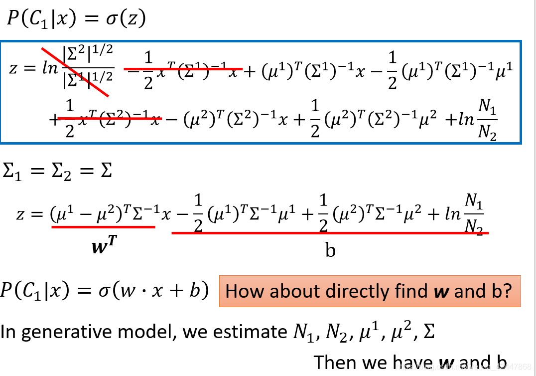
Generative model方法跟Logistic regression方法类似，不同之处在于Generative model可以直接计算出w和b的最佳解，而Logistic regression是将w和b进行初始化，通过迭代训练来更新w和b

代码除了求解w和b地方不一样，其他地方类似，完整代码如下

import numpy as np

np.random.seed(0)

#添加文件路径
X_train_fpath = 'E:/jupyter/data/hw2/data/X_train'
Y_train_fpath = 'E:/jupyter/data/hw2/data/Y_train'
X_test_fpath = 'E:/jupyter/data/hw2/data/X_test'
output_fpath = 'E:/jupyter/work2/output_{}.csv'
#归一化
def _normalize(X, train = True, specified_column = None, X_mean = None, X_std = None):
   
    if specified_column == None:
        #为每个数据添加索值
        specified_column = np.arange(X.shape[1])
    if train:
        #求取每个数据的平均值和标准差
        X_mean = np.mean(X[:, specified_column] ,0).reshape(1,-1)
        X_std  = np.std(X[:, specified_column], 0).reshape(1,-1)
    #归一化数据
    X[:,specified_column] = (X[:, specified_column] - X_mean) / (X_std + 1e-8)
     #返回归一化后的数据，均值，标准差
    return X, X_mean, X_std
# Parse csv files to numpy array
with open(X_train_fpath) as f:
    next(f)
    X_train = np.array([line.strip('\n').split(',')[1:] for line in f], dtype = float)
with open(Y_train_fpath) as f:
    next(f)
    Y_train = np.array([line.strip('\n').split(',')[1] for line in f], dtype = float)
with open(X_test_fpath) as f:
    next(f)
    X_test = np.array([line.strip('\n').split(',')[1:] for line in f], dtype = float)

# Normalize training and testing data
X_train, X_mean, X_std = _normalize(X_train, train = True)
X_test, _, _= _normalize(X_test, train = False, specified_column = None, X_mean = X_mean, X_std = X_std)
# Compute in-class mean
X_train_0 = np.array([x for x, y in zip(X_train, Y_train) if y == 0])
X_train_1 = np.array([x for x, y in zip(X_train, Y_train) if y == 1])

mean_0 = np.mean(X_train_0, axis = 0)
mean_1 = np.mean(X_train_1, axis = 0)  
data_dim = X_train.shape[1]
# Compute in-class covariance
cov_0 = np.zeros((data_dim, data_dim))
cov_1 = np.zeros((data_dim, data_dim))

for x in X_train_0:
    cov_0 += np.dot(np.transpose([x - mean_0]), [x - mean_0]) / X_train_0.shape[0]
for x in X_train_1:
    cov_1 += np.dot(np.transpose([x - mean_1]), [x - mean_1]) / X_train_1.shape[0]

# Shared covariance is taken as a weighted average of individual in-class covariance.
cov = (cov_0 * X_train_0.shape[0] + cov_1 * X_train_1.shape[0]) / (X_train_0.shape[0] + X_train_1.shape[0])
#sigmoid函数
def _sigmoid(z):
    # Sigmoid function can be used to calculate probability.
    # To avoid overflow, minimum/maximum output value is set.
    return np.clip(1 / (1.0 + np.exp(-z)), 1e-8, 1 - (1e-8))
#向前传播然后利用sigmoid激活函数计算激活值
def _f(X, w, b):
    return _sigmoid(np.matmul(X, w) + b)
#准确度
def _accuracy(Y_pred, Y_label):
    # This function calculates prediction accuracy
    acc = 1 - np.mean(np.abs(Y_pred - Y_label))
    return acc
#预测
def _predict(X, w, b):
    return np.round(_f(X, w, b)).astype(np.int)
# Compute inverse of covariance matrix.
# Since covariance matrix may be nearly singular, np.linalg.inv() may give a large numerical error.
# Via SVD decomposition, one can get matrix inverse efficiently and accurately.
u, s, v = np.linalg.svd(cov, full_matrices=False)
inv = np.matmul(v.T * 1 / s, u.T)

# Directly compute weights and bias
w = np.dot(inv, mean_0 - mean_1)
b =  (-0.5) * np.dot(mean_0, np.dot(inv, mean_0)) + 0.5 * np.dot(mean_1, np.dot(inv, mean_1))\
    + np.log(float(X_train_0.shape[0]) / X_train_1.shape[0]) 

# Compute accuracy on training set
Y_train_pred = 1 - _predict(X_train, w, b)
print('Training accuracy: {}'.format(_accuracy(Y_train_pred, Y_train)))

运行之后

Training accuracy: 0.8718114125626659

我的运行结果显示，利用Generative model在训练集上的准确度为87.18%，感觉和Logistic regression差不多

下面是计算w和b的原理图，由最大似然估计和贝叶斯公式推导而来，有兴趣的同学可以自己按照视频内容推导一下
有错误的地方希望大家批评指正，谢谢！