MATLAB郭彦甫进阶绘图

瑶啊瑶啊露

已于 2024-01-02 11:31:07 修改

阅读量872

点赞数 22

分类专栏： matlab 文章标签： matlab

于 2023-12-27 16:42:33 首次发布

本文链接：https://blog.csdn.net/weixin_42530996/article/details/135229024

版权

matlab 专栏收录该内容

1 篇文章 0 订阅

订阅专栏

MATLAB 进阶绘图

二维图表
三维图表

写论文过程中，发现仿真还存在很大的问题，遂学习了郭彦甫老师的MATLAB画图部分，将PPT中的代码重新复现仿真跑了一遍，仅供学习参考。

二维图表

函数	图形描述
loglog()	x轴和y轴都取对数坐标
semilogx()	x轴取对数坐标，y轴取线性坐标
semilogy()	x轴取线性坐标，y轴取对数坐标
plotyy()	带有两套y坐标轴的线性坐标系
ploar()	极坐标系
hist()	直方图
bar()	二维柱状图
pie()	饼图
stairs	阶梯图
stem()	针状图

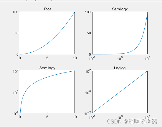
对数坐标系图线 - logarithm plots

x = logspace(-1,1,100); 
y = x.^2;
subplot(2,2,1);
plot(x,y);
title('Plot');

subplot(2,2,2);
semilogx(x,y);
title('Semilogx');

subplot(2,2,3);
semilogy(x,y);
title('Semilogy');

subplot(2,2,4);
loglog(x, y);
title('Loglog');

在这里插入图片描述
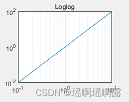
对坐标系加上网格，以区分线性坐标系与对数坐标系

set(gca, 'XGrid','on');

在这里插入图片描述

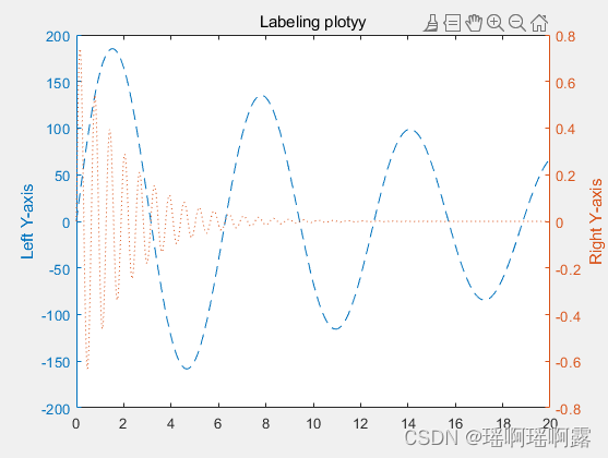
双y轴曲线 - plotyy

x = 0:0.01:20;
y1 = 200*exp(-0.05*x).*sin(x);
y2 = 0.8*exp(-0.5*x).*sin(10*x);
[AX,H1,H2] = plotyy(x,y1,x,y2);
set(get(AX(1),'Ylabel'),'String','Left Y-axis')
set(get(AX(2),'Ylabel'),'String','Right Y-axis')
title('Labeling plotyy');
set(H1,'LineStyle','--'); set(H2,'LineStyle',':');

在这里插入图片描述

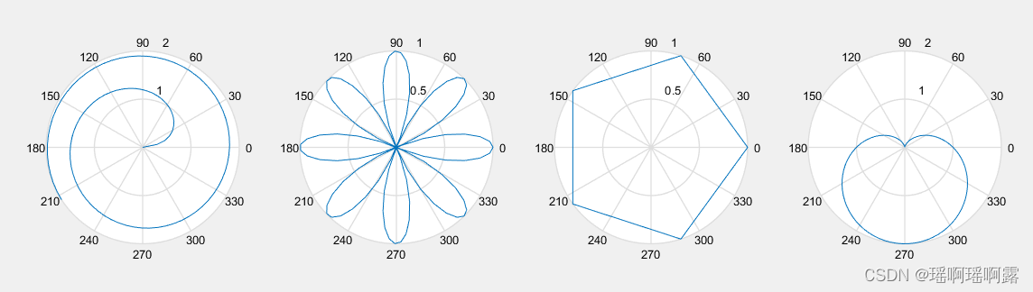
极坐标图 - polar

% 螺旋线
x = 1:100; 
theta = x/10;
 r = log10(x);
subplot(1,4,1); 
polar(theta,r);

% 花瓣
theta = linspace(0, 2*pi); 
r = cos(4*theta);
subplot(1,4,2); 
polar(theta, r);

% 五边形
theta = linspace(0, 2*pi, 6); 
r = ones(1,length(theta));
subplot(1,4,3); 
polar(theta,r);

% 心形线
theta = linspace(0, 2*pi);
 r = 1-sin(theta);
subplot(1,4,4); 
polar(theta , r);

在这里插入图片描述

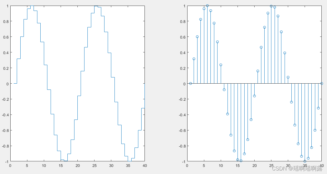
阶梯图和针状图-Stairs and Stem Charts

用来表示离散的数字序列

x = linspace(0, 4*pi, 40);
 y = sin(x);
subplot(1,2,1); stairs(y);
subplot(1,2,2); stem(y);

在这里插入图片描述

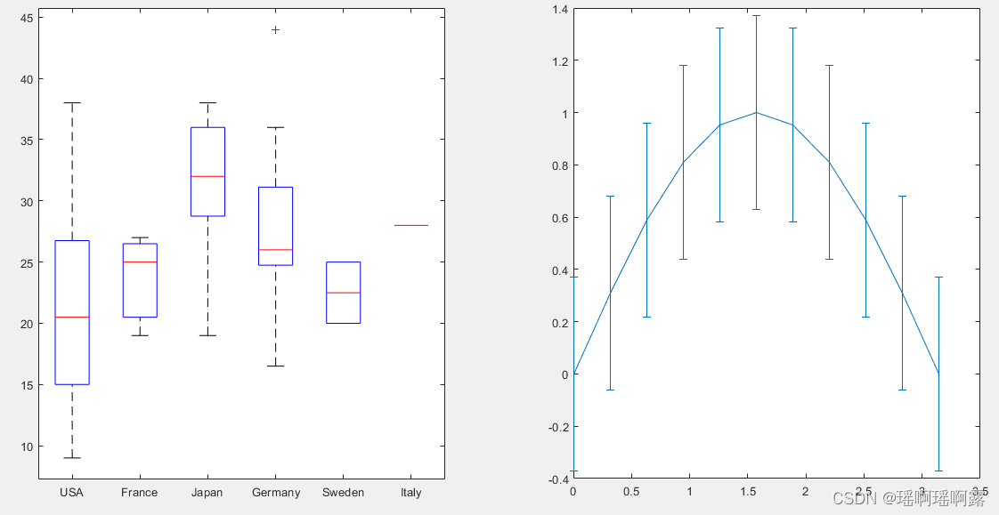
Boxplot and Error Bar

load carsmall
subplot(1,2,1);
boxplot(MPG, Origin);

x=0:pi/10:pi; 
y=sin(x);
e=std(y)*ones(size(x));
subplot(1,2,2);
errorbar(x,y,e)

在这里插入图片描述

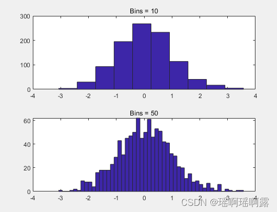
直方图-Histogram

多用于查看变量的频率分布

x = randn(1,1000);
subplot(2,1,1);
hist(x,10);
title('Bins = 10');
subplot(2,1,2);
hist(x,50); 
title('Bins = 50');

%hist(x,nbins) x表示原始数据，nbins表示分组的个数

在这里插入图片描述

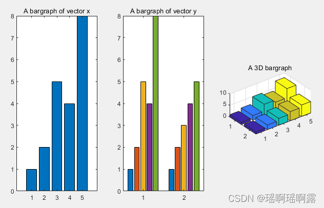
柱状图-Bar Charts

多用于查看分立的量的统计结果

x = [1 2 5 4 8]; 
y = [x;1:5];
subplot(1,3,1); 
bar(x); 
title('A bargraph of vector x');
subplot(1,3,2); 
bar(y);
 title('A bargraph of vector y');
subplot(1,3,3); 
bar3(y);
title('A 3D bargraph');

在这里插入图片描述

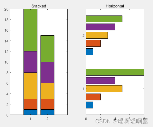
bar()传入‘stack’参数可以让柱状图以堆栈的形式画出
barh()函数可以绘制纵向排列的柱状图

x = [1 2 5 4 8];
y = [x;1:5];
subplot(1,2,1);
bar(y,'stacked');
title('Stacked');
subplot(1,2,2);
barh(y);
title('Horizontal');

在这里插入图片描述

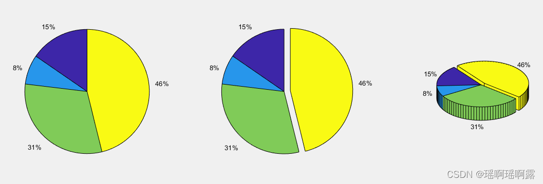
饼图 - pie charts

a = [10 5 20 30];
subplot(1,3,1); pie(a);
subplot(1,3,2); pie(a, [0,0,0,1]);
subplot(1,3,3); pie3(a, [0,0,0,1]);

在这里插入图片描述

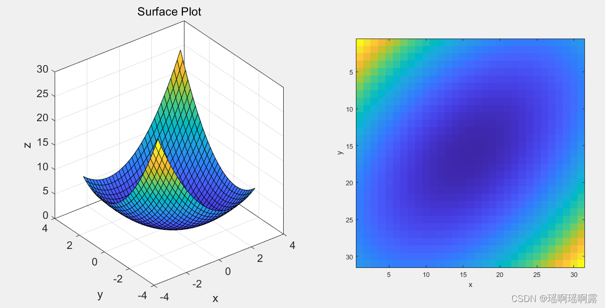
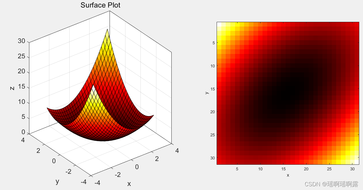
三维图表

将数据可视化为图像


[x, y] = meshgrid(-3:0.2:3, -3:0.2:3);
z = x.^2 + x.*y + y.^2; 
subplot(1,2,1);
surf(x, y, z);

box on;
set(gca,'FontSize',16);
zlabel('z');
xlim([-4,4]); xlabel('x');
ylim([-4,4]);ylabel('y');             %画出一个立体图形
title('Surface Plot');

subplot(1,2,2);
imagesc(z);%将数据可视化为图像
axis square;
xlabel('x');
ylabel('y');

在这里插入图片描述

colorbar可以在生成的图上增加颜色和高度间对应关系的图例
在这里插入图片描述

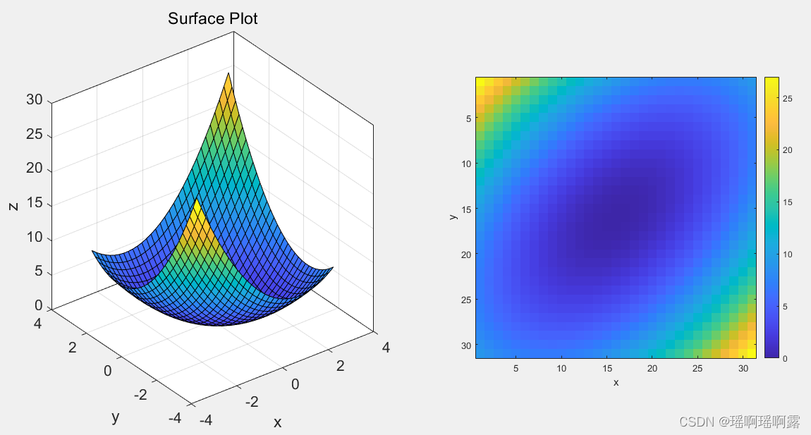
colormap命令可以改变配色方案

colormap(hot)

在这里插入图片描述

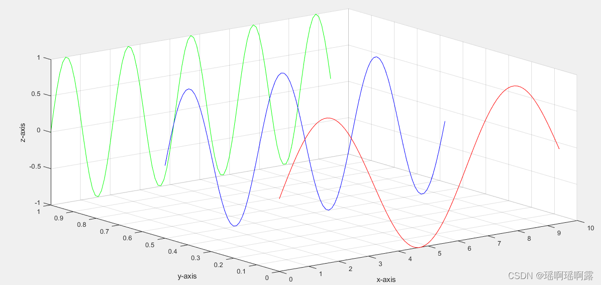
绘制三维线 - 3D Line Plots

x=0:0.1:3*pi; 
z1=sin(x);  z2=sin(2.*x);  z3=sin(3.*x);
y1=zeros(size(x)); y3=ones(size(x)); y2=y3./2;
plot3(x,y1,z1,'r',x,y2,z2,'b',x,y3,z3,'g'); grid on;
xlabel('x-axis'); ylabel('y-axis'); zlabel('z-axis');

在这里插入图片描述

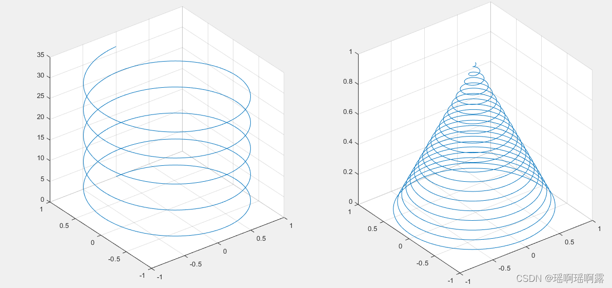
其他的3维的线图

subplot(1, 2, 1)
t = 0:pi/50:10*pi;
plot3(sin(t),cos(t),t)
grid on; axis square;

subplot(1, 2, 2)
turns = 40*pi;
t = linspace(0,turns,4000);
x = cos(t).*(turns-t)./turns;
y = sin(t).*(turns-t)./turns;
z = t./turns;
plot3(x,y,z); grid on;

在这里插入图片描述

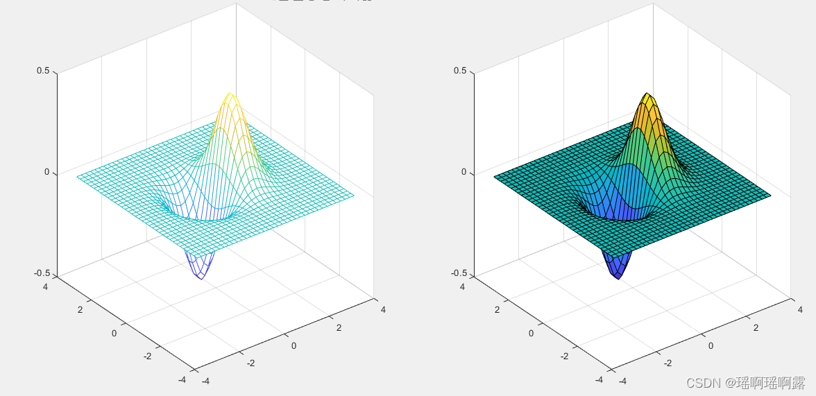
绘制三维面 - 3D Surface Plots

meshgrid()生成二维网格

x = -2:1:2;
y = -2:1:2;
[X,Y] = meshgrid(x,y)
Z = X.^2 + Y.^2

X =
    -2    -1     0     1     2
    -2    -1     0     1     2
    -2    -1     0     1     2
    -2    -1     0     1     2
    -2    -1     0     1     2


Y =
    -2    -2    -2    -2    -2
    -1    -1    -1    -1    -1
     0     0     0     0     0
     1     1     1     1     1
     2     2     2     2     2
     
Z =
     8     5     4     5     8
     5     2     1     2     5
     4     1     0     1     4
     5     2     1     2     5
     8     5     4     5     8

mesh()和surf()命令都可以绘制三维面，前者不会填充网格，后者会

x = -3.5:0.2:3.5;
y = -3.5:0.2:3.5;
[X,Y] = meshgrid(x,y);
Z = X.*exp(-X.^2-Y.^2);
subplot(1,2,1); mesh(X,Y,Z);
subplot(1,2,2); surf(X,Y,Z);

在这里插入图片描述

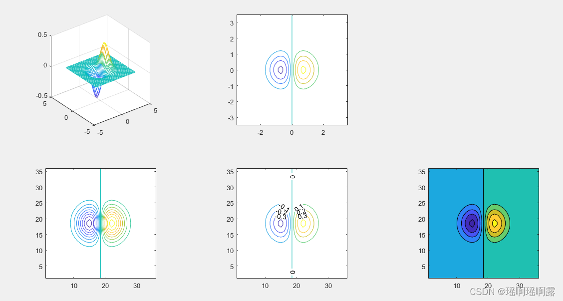
绘制等高线- contour()

contour()绘制函数等高线
向contour()函数传入参数或操作图形句柄可以改变图像的细节

x = -3.5:0.2:3.5;
y = -3.5:0.2:3.5;
[X,Y] = meshgrid(x,y);
Z = X.*exp(-X.^2-Y.^2);

subplot(2,3,1);mesh(X,Y,Z); axis square;
subplot(2,3,2);contour(X,Y,Z); axis square;
subplot(2,3,4); contour(Z,[-.45:.05:.45]); axis square;
subplot(2,3,5); [C,h] = contour(Z); clabel(C,h); axis square;
subplot(2,3,6); contourf(Z); axis square;

在这里插入图片描述
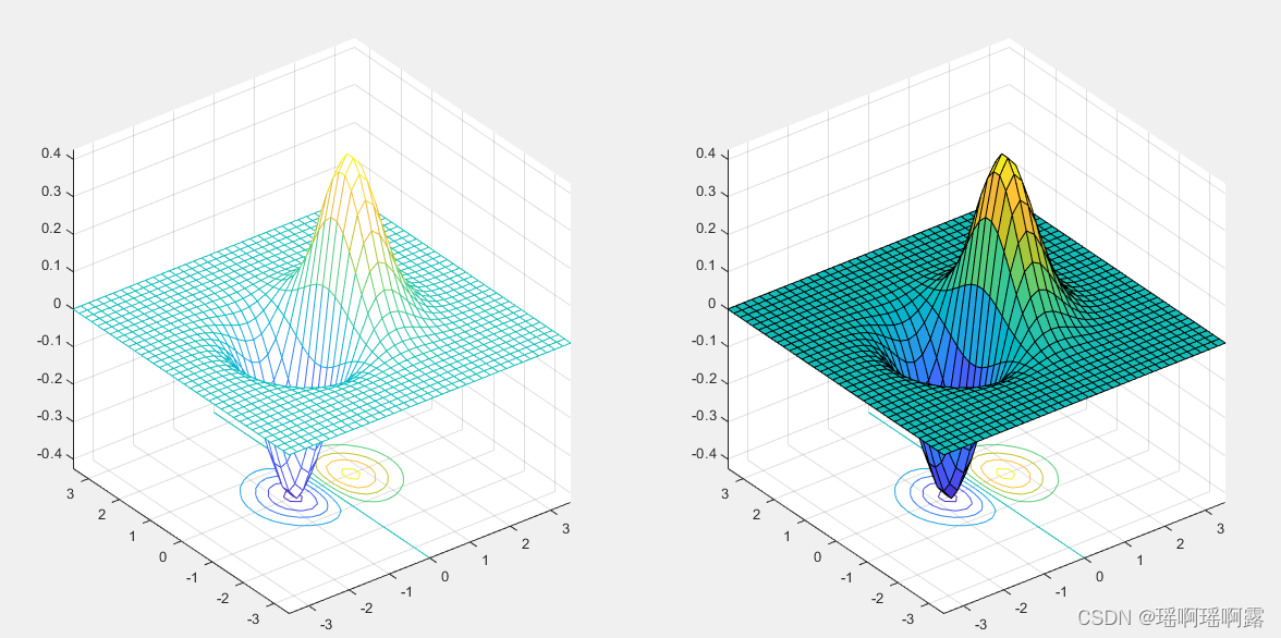
meshc()和surfc()可以同时绘制三维图形及其等高线

x = -3.5:0.2:3.5; y = -3.5:0.2:3.5;
[X,Y] = meshgrid(x,y); Z = X.*exp(-X.^2-Y.^2);

subplot(1,2,1); meshc(X,Y,Z);
subplot(1,2,2); surfc(X,Y,Z);

在这里插入图片描述

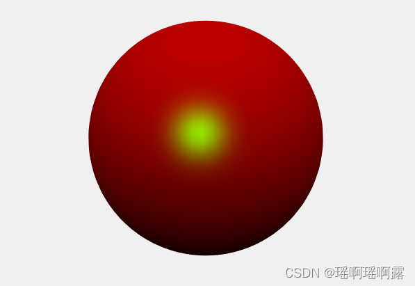
三维图的角度与光线 - view()和light()

[X, Y, Z] = sphere(64); 
h = surf(X, Y, Z);
axis square vis3d off;
reds = zeros(256, 3); 
reds(:, 1) = (0:256.-1)/255;
colormap(reds); shading interp; lighting phong;
set(h, 'AmbientStrength', 0.75, 'DiffuseStrength', 0.5);
L1 = light('Position', [-1, -1, -1])
set(L1, 'Position', [-1, -1, 1]);
set(L1, 'Color', 'g');

在这里插入图片描述

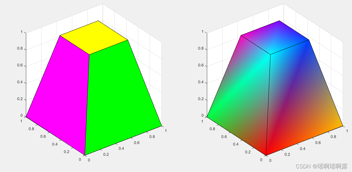
绘制三维多边形 - patch（）

patch()

v = [0 0 0; 1 0 0 ; 1 1 0; 0 1 0; 0.25 0.25 1; 0.75 0.25 1; 0.75 0.75 1; 0.25 0.75 1];
f = [1 2 3 4; 5 6 7 8; 1 2 6 5; 2 3 7 6; 3 4 8 7; 4 1 5 8];

subplot(1,2,1); 
patch('Vertices', v, 'Faces', f, 'FaceVertexCData', hsv(6), 'FaceColor', 'flat');
view(3); axis square tight; grid on;

subplot(1,2,2); 
patch('Vertices', v, 'Faces', f, 'FaceVertexCData', hsv(8), 'FaceColor','interp');
view(3); axis square tight; grid on

在这里插入图片描述