


背景点源呈现二维高斯轮廓。可以使用二维高斯拟合去除,效果如下图红色框框住的部分。需要每个点源的位置坐标,然后把位置坐标写成csv文件,即可对每个点源的循环去除。练习文件下载地址点击这里下载。另外也可以在本人博客下载区域,已经把csv文件、代码和练习文件全部打包成压缩包。代码参考下文
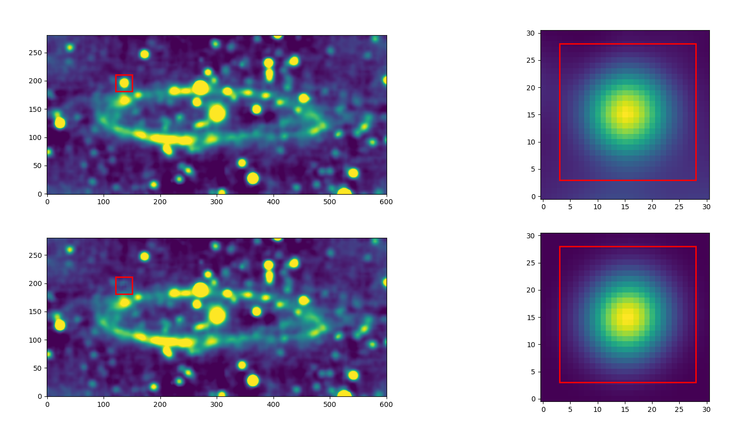
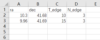
背景点源的csv格式。其中T_edge是指高斯点源拟合区域的大小,10即以10个pix的大小。N_edge是指周围背景的大小,即把T_edge+N_edge = 13,13*13矩阵四周延伸3个pix的区域作为背景拟合。
#!/usr/bin/env python

import numpy as np
from astropy.modeling import Fittable2DModel, Parameter, models, fitting
from astropy.io import fits as pf
import matplotlib.pyplot as plt
import os
import sys
from astropy.wcs import WCS
import pandas as pd
import matplotlib.patches as patches


source_position = pd.read_csv('backourd_source.csv')   #背景点源文件
check_data = True  #首先要对每个点源检查,就打开。等到背景点源文件记录完毕了,再改成FALSE
inf = 'BHJ_cite_map_H.fits'  #练习文件,只有两个轴
data = pf.getdata(inf)

for key in range(source_position.shape[0]):
    print(key)
    df = source_position[key:key+1]
    center_word= [float(df['ra']), float(df['dec'])]   #背景源的大致位置
    T_edge = int(df['T_edge'])
    N_edge = int(df['N_edge'])

    if check_data:
        df = [10.3, 41.68, 15, 3]   #逐个点检查,前面两个是ra和dec 后面是T_edge和N_edge。
        center_word = [df[0],df[1]]
        T_edge = df[2]
        N_edge = df[3]

    if not os.path.exists(inf): continue

    hdr = pf.getheader(inf)
    wn = WCS(hdr)
    grid = abs(hdr['CDELT1'])
    x, y = np.mgrid[0:data.shape[0],0:data.shape[1]]
    y = hdr['CRVAL1']+(1-hdr['CRPIX1'])*hdr['CDELT1']-y*grid   # gl
    x = hdr['CRVAL2']+(1-hdr['CRPIX2'])*hdr['CDELT2']+x*grid   # gb


    pix = wn.all_world2pix([center_word], 0)[0]
    xs = int(pix[0])
    ys = int(pix[1])


    s_edge = int(T_edge/2)
    search_data = data[ys-s_edge:ys+s_edge, xs-s_edge:xs+s_edge]
    y0, x0 = np.where(data==search_data.max())


    fit_data = data[y0[0]-T_edge:y0[0]+T_edge+1, x0[0]-T_edge:x0[0]+T_edge+1]
    fit_y = y[y0[0]-T_edge:y0[0]+T_edge+1, x0[0]-T_edge:x0[0]+T_edge+1]
    fit_x = x[y0[0]-T_edge:y0[0]+T_edge+1, x0[0]-T_edge:x0[0]+T_edge+1]

    if check_data:

        fig1 = plt.figure(1)
        ax1 = fig1.add_subplot(221)
        ax2 = fig1.add_subplot(222)
        ax3 = fig1.add_subplot(223)
        ax4 = fig1.add_subplot(224)

        vmax = np.percentile(data,97)
        vmin = np.percentile(data,5)
        ax1.imshow(data, origin = 'lower', vmax = vmax, vmin = vmin)
        ax2.imshow(fit_data, origin='lower')
        N = fit_data.shape[0]

        rect1 = patches.Rectangle((x0[0]-T_edge, y0[0]-T_edge), 2*T_edge, 2*T_edge, linewidth=2, edgecolor='r', facecolor='none')

        ax1.add_patch(rect1)
        rect2 = patches.Rectangle((N_edge, N_edge), N-2*N_edge, N-2*N_edge, linewidth=2, edgecolor='r', facecolor='none')
        ax2.add_patch(rect2)


    fit_data0 = np.zeros_like(fit_data)
    fit_data0[N_edge:-N_edge, N_edge:-N_edge] = 1.

    word = wn.all_pix2world([[x0[0], y0[0]]],0)[0]
    x_mean = word[0]
    y_mean = word[1]

    y_mean = np.median(fit_x)
    x_mean = np.median(fit_y)
    x_std = 0.05
    y_std = 0.05


    p_init = models.Polynomial2D(1)
    p_init.c0_0 = np.median(fit_data[fit_data0<0.5])     #背景数据


    ytt = fit_data - p_init.c0_0
    #ytt[fit_data0<0.5]=0.
    amp = np.max(ytt)
    ind = np.unravel_index(np.argmax(ytt, axis=None), ytt.shape)
    g_init = models.Gaussian2D(amplitude=amp, x_mean=x_mean, y_mean=y_mean, x_stddev=x_std, y_stddev=y_std)

    pg = p_init + g_init
    fit = fitting.LevMarLSQFitter()
    fitted_model = fit(pg, fit_y, fit_x, fit_data)

    Intensity = fitted_model[1].amplitude.value
    x_beam = fitted_model[1].x_stddev.value*2.*np.sqrt(2.*np.log(2.))*60.
    y_beam = fitted_model[1].y_stddev.value*2.*np.sqrt(2.*np.log(2.))*60.
    theta = fitted_model[1].theta.value
    x_mean = fitted_model[1].x_mean.value
    y_mean = fitted_model[1].y_mean.value

    '''
    ss = key + '  ' + Dict[key] + '  ' + str(Intensity) + '  ' + str(x_beam)+ '  ' + str(y_beam) + '  ' + str(theta) + '  ' + str(x_mean) + '  ' + str(y_mean) +'  ' + str(amp) + '  ' + str(y[ind]) + '  ' + str(x[ind]) + '\n'
    print(ss)
    f.write(ss)
    '''
    #这里注释掉了很多信息,如果你需要可以逐个打印出来

    data[y0[0]-T_edge:y0[0]+T_edge+1, x0[0]-T_edge:x0[0]+T_edge+1] = fit_data - fitted_model[1](fit_y, fit_x)

    if check_data:
        ax3.imshow(data, origin = 'lower', vmax = vmax, vmin = vmin)
        ax4.imshow(fitted_model[1](fit_y, fit_x), origin = 'lower')

        rect3 = patches.Rectangle((x0[0]-T_edge, y0[0]-T_edge), 2*T_edge, 2*T_edge, linewidth=2, edgecolor='r', facecolor='none')
        ax3.add_patch(rect3)
        rect4 = patches.Rectangle((N_edge, N_edge), N-2*N_edge, N-2*N_edge, linewidth=2, edgecolor='r', facecolor='none')
        ax4.add_patch(rect4)
        plt.show()
        sys.exit()   #如果是逐个点的检查模式,那么检查完一个点就结束程序。

ouf = inf.replace('.fits', '_diff.fits')
pf.writeto(ouf, data , hdr, overwrite=True)
 #最后生成后缀带有_diff的文件即为已经去除了背景点源的fist文件
#ouf = inf.replace('.fits', '_model.fits')
#pf.writeto(ouf, fitted_model[1](fit_y, fit_x), hdr, overwrite=True)


 1万+
1万+


 被折叠的 条评论
为什么被折叠?
被折叠的 条评论
为什么被折叠?
 到【灌水乐园】发言


