[c++][SDL]图形学菜鸡的软渲染之路3-矩阵与各种变换

矩阵变换

矩阵的调用顺序和作用可以参考之前的博客：
渲染流程概述

线性代数相关数学知识可以参考
https://www.bilibili.com/video/av6731067/?p=13

我们的模型矩阵，视图矩阵，投影矩阵大小都是4x4的。
为了让一个三维的顶点坐标可以4x4的矩阵进行运算，必须先让他变成四维的，及齐次化，增加维度w。一个齐次化坐标(x, y, z, w)，和世界坐标(x,y,z)的关系是：$$\left(\begin{array}{c}\frac{x}{w},\frac{y}{w},\frac{z}{w}\end{array}\right)=\left(\begin{array}{c}x,y,z\end{array}\right)$$

1.模型矩阵

这里所有矩阵的使用方法都是矩阵左乘一个向量

平移矩阵

在三维空间中，一个顶点(x, y, z)平移(a, b, c)的结果是(x + a, y + b, z + c)这一变换用矩阵表达为：
$$\left[\begin{array}{cccc}1& 0& 0& a\\ 0& 1& 0& b\\ 0& 0& 1& c\\ 0& 0& 0& 1\end{array}\right]\ast \left[\begin{array}{c}x\\ y\\ z\\ 1\end{array}\right]=\left[\begin{array}{c}x+a\\ y+b\\ z+c\\ 1\end{array}\right]$$

Matrix translate(double x, double y, double z) {
	Matrix t;
	t = Matrix::identity();
	t[0][3] = x;
	t[1][3] = y;
	t[2][3] = z;
	return t;
};

缩放矩阵

在三维空间中，一个顶点(x, y, z)以坐标原点(0,0,0)为中心,各个方向缩放(a, b, c)的结果是(x * a, y * b, z * c)这一变换用矩阵表达为：
$$\left[\begin{array}{cccc}a& 0& 0& 0\\ 0& b& 0& 0\\ 0& 0& c& 0\\ 0& 0& 0& 1\end{array}\right]\ast \left[\begin{array}{c}x\\ y\\ z\\ 1\end{array}\right]=\left[\begin{array}{c}x\ast a\\ y\ast b\\ z\ast c\\ 1\end{array}\right]$$

Matrix scale(double x, double y, double z) {
	Matrix t;
	t= Matrix::identity();
	t[0][0] = x;
	t[1][1] = y;
	t[2][2] = z;
	return t;
};

旋转矩阵

Reference：
旋转变换（一）旋转矩阵
常用三角函数公式

二维情况

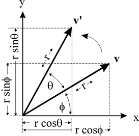
如图所示点v 绕 原点旋转θ 角，设v到原点距离为r，
则v的坐标为$$(r\ast cos(\varphi ),r\ast sin(\varphi ))$$

旋转后v‘坐标为$$(r\ast cos(\theta +\varphi ),r\ast sin(\theta +\varphi ))$$

通过两角和公式展开得：v‘坐标为

$$(r\ast cos\theta cos\varphi -r\ast sin\theta sin\varphi ,r\ast sin\theta cos\varphi +r\ast cos\theta sin\varphi )$$

代入v点表达式得：$$(x\ast cos\varphi -y\ast sin\varphi ,y\ast cos\varphi +x\ast sin\varphi )$$

即
$$x\prime =xcos\theta -ysin\theta$$

$$y\prime =xsin\theta +ycos\theta$$

用矩阵表达为:
$$\left[\begin{array}{c}{x}^{\prime }\\ y^{\prime }\end{array}\right]=\left[\begin{array}{cc}cos\theta & -sin\theta \\ sin\theta & cos\theta \end{array}\right]\ast \left[\begin{array}{c}x\\ y\end{array}\right]$$

绕任意点的二维旋转

我们可以三部把绕任意点的情况转换为绕原点旋转的情况：

1. 首先将旋转点移动到原点处
2. 执行绕原点的旋转
3. 再将旋转点移回到原来的位置
   

平移矩阵我们前面已经介绍过了，现在设点绕t(x,y)旋转θ度，则复合旋转矩阵为：
$$\left[\begin{array}{ccc}1& 0& t.x\\ 0& 1& t.y\\ 0& 0& 1\end{array}\right]\ast \left[\begin{array}{ccc}cos\theta & -sin\theta & 0\\ sin\theta & cos\theta & 0\\ 0& 0& 1\end{array}\right]\ast \left[\begin{array}{ccc}1& 0& -t.x\\ 0& 1& -t.y\\ 0& 0& 1\end{array}\right]$$

$$=\left[\begin{array}{ccc}cos\theta & -sin\theta & t.x\\ sin\theta & cos\theta & t.y\\ 0& 0& 1\end{array}\right]\ast \left[\begin{array}{ccc}1& 0& -t.x\\ 0& 1& -t.y\\ 0& 0& 1\end{array}\right]$$

$$=\left[\begin{array}{ccc}cos\theta & -sin\theta & -t.x\ast cos\theta +t.y\ast sin\theta +t.x\\ sin\theta & cos\theta & -t.x\ast sin\theta -t.y\ast cos\theta +t.y\\ 0& 0& 1\end{array}\right]$$

$$=\left[\begin{array}{ccc}cos\theta & -sin\theta & (1-cos\theta )\ast t.x+t.y\ast sin\theta \\ sin\theta & cos\theta & (1-sin\theta )\ast t.y-t.x\ast sin\theta \\ 0& 0& 1\end{array}\right]$$

三维基本旋转

1.绕坐标轴旋转

这里我们旋转方向用右手坐标系定义

绕z轴旋转其实就是在xoy面上进行旋转，与我们的二维情况完全相同，可以直接套用我们刚刚推出的二维旋转公式。
$$\left[\begin{array}{c}{x}^{\prime }\\ y^{\prime }\\ z^{\prime }\\ 1\end{array}\right]=\left[\begin{array}{cccc}cos\theta & -sin\theta & 0& 0\\ sin\theta & cos\theta & 0& 0\\ 0& 0& 1& 0\\ 0& 0& 0& 1\end{array}\right]\ast \left[\begin{array}{c}x\\ y\\ z\\ 1\end{array}\right]$$
绕x轴旋转为在yoz面上旋转，y轴类似二维情况的x轴，z轴为二维情况的y轴，符合右手方向，同样可以套用我们之前推出的公式：
$$\left[\begin{array}{c}{x}^{\prime }\\ y^{\prime }\\ z^{\prime }\\ 1\end{array}\right]=\left[\begin{array}{cccc}1& 0& 0& 0\\ 0& cos\theta & -sin\theta & 0\\ 0& sin\theta & cos\theta & 0\\ 0& 0& 0& 1\end{array}\right]\ast \left[\begin{array}{c}x\\ y\\ z\\ 1\end{array}\right]$$
绕y轴旋转为在zox面上旋转，z轴类似二维情况的x轴，x轴为二维情况的y轴，即：
x′=zsinθ+xcosθ
y′=y
z′=zcosθ−xsinθ
可以得到矩阵
$$\left[\begin{array}{c}{x}^{\prime }\\ y^{\prime }\\ z^{\prime }\\ 1\end{array}\right]=\left[\begin{array}{cccc}cos\theta & 0& sin\theta & 0\\ 0& 1& 0& 0\\ -sin\theta & 0& cos\theta & 0\\ 0& 0& 0& 1\end{array}\right]\ast \left[\begin{array}{c}x\\ y\\ z\\ 1\end{array}\right]$$

2.绕任意轴旋转

推导方法一：

类似与二维时绕任意点旋转，我们同样可以把绕任意轴的旋转分解成绕三个坐标轴分别旋转。假设现在有一个点P要绕向量u旋转θ角度，得到点Q，求Q的步骤如下：

1. 将旋转轴u绕x轴旋转至xoz平面
2. 将旋转轴u绕y轴旋转至于z轴重合
3. 绕z轴旋转θ角
4. 执行步骤2的逆过程
5. 执行步骤1的逆过程
   过程：
   
   u为旋转轴，作点P在yoz平面的投影点q，q的坐标是（0, b, c)，原点o与q点的连线oq和z轴的夹角α就是u绕x轴旋转的角度。通过这次旋转使得u向量旋转到xoz平面（图中的or向量）【步骤1】
   过r点作z轴的垂线，or与z轴的夹角为β, 这个角度就是绕Y轴旋转的角度，通过这次旋转使得u向量旋转到与z轴重合【步骤2】

步骤一绕x轴旋转α度的旋转矩阵为：
$$\left[\begin{array}{cccc}1& 0& 0& 0\\ 0& cos\alpha & -sin\alpha & 0\\ 0& sin\alpha & cos\alpha & 0\\ 0& 0& 0& 1\end{array}\right]$$
由图片可以得到，$$cos\alpha =\frac{c}{\sqrt{b^2+c^2}}$$

$$sin\alpha =\frac{b}{\sqrt{b^2+c^2}}$$

记第一步旋转矩阵Rx(α) ,代入数据得：
$$\left[\begin{array}{cccc}1& 0& 0& 0\\ 0& \frac{c}{\sqrt{(b^2+c^2)}}& -\frac{b}{\sqrt{(b^2+c^2)}}& 0\\ 0& \frac{b}{\sqrt{(b^2+c^2)}}& \frac{c}{\sqrt{(b^2+c^2)}}& 0\\ 0& 0& 0& 1\end{array}\right]$$
逆变换Rx(-α)为：
$$\left[\begin{array}{cccc}1& 0& 0& 0\\ 0& cos\alpha & sin\alpha & 0\\ 0& -sin\alpha & cos\alpha & 0\\ 0& 0& 0& 1\end{array}\right]=\left[\begin{array}{cccc}1& 0& 0& 0\\ 0& \frac{c}{\sqrt{(b^2+c^2)}}& \frac{b}{\sqrt{(b^2+c^2)}}& 0\\ 0& -\frac{b}{\sqrt{(b^2+c^2)}}& \frac{c}{\sqrt{(b^2+c^2)}}& 0\\ 0& 0& 0& 1\end{array}\right]$$

在完成步骤1之后，向量u被变换到了r的位置，我们继续步骤2的操作，绕y轴旋转负的β角（注意：这里的β是负的，因为我们按照右手方向进行旋转），经过这次变换之后向量u与z轴完全重合，由于这一步也是执行的一次绕Y轴的基本旋转，旋转矩阵（记作 Ry(−β))为：
$$\left[\begin{array}{cccc}cos\beta & 0& sin\beta & 0\\ 0& 1& 0& 0\\ -sin\beta & 0& cos\beta & 0\\ 0& 0& 0& 1\end{array}\right]$$

其中$$cos\beta =\frac{\sqrt{(b^2+c^2)}}{\sqrt{(a^2+b^2+c^2)}}$$

$$sin\beta =\frac{a}{\sqrt{(a^2+b^2+c^2)}}$$

记第二步旋转矩阵Ry(-β) ,代入数据得：
$$\left[\begin{array}{cccc}cos(-\beta )& 0& sin(-\beta )& 0\\ 0& 1& 0& 0\\ -sin(-\beta )& 0& cos(-\beta )& 0\\ 0& 0& 0& 1\end{array}\right]=\left[\begin{array}{cccc}cos\beta & 0& -sin\beta & 0\\ 0& 1& 0& 0\\ sin\beta & 0& cos\beta & 0\\ 0& 0& 0& 1\end{array}\right]$$

$$=\left[\begin{array}{cccc}\frac{\sqrt{(b^2+c^2)}}{\sqrt{(a^2+b^2+c^2)}}& 0& -\frac{a}{\sqrt{a^2+b^2+c^2}}& 0\\ 0& 1& 0& 0\\ \frac{a}{\sqrt{(a^2+b^2+c^2)}}& 0& \frac{\sqrt{(b^2+c^2)}}{\sqrt{(a^2+b^2+c^2)}}& 0\\ 0& 0& 0& 1\end{array}\right]$$
逆变换Ry(β)为：
$$\left[\begin{array}{cccc}cos\beta & 0& sin\beta & 0\\ 0& 1& 0& 0\\ -sin\beta & 0& cos\beta & 0\\ 0& 0& 0& 1\end{array}\right]=\left[\begin{array}{cccc}\frac{\sqrt{(b^2+c^2)}}{\sqrt{(a^2+b^2+c^2)}}& 0& \frac{a}{\sqrt{(a^2+b^2+c^2)}}& 0\\ 0& 1& 0& 0\\ -\frac{a}{\sqrt{(a^2+b^2+c^2)}}& 0& \frac{\sqrt{(b^2+c^2)}}{\sqrt{(a^2+b^2+c^2)}}& 0\\ 0& 0& 0& 1\end{array}\right]$$
最终得到 绕任意轴u旋转的旋转矩阵是【因为使用的列向量，因此执行的是左乘（从右往左）】：
$$MR=Rx(-\alpha )\ast Ry(\beta )\ast Rz(\theta )\ast Ry(-\beta )\ast Rx(\alpha )=$$
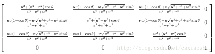
其中(u, v, w)对应上文(a,b,c),如果旋转轴向量时单位化的，矩阵可以化简为：

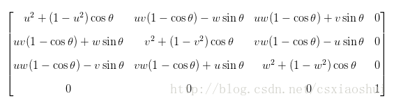
推导方法二：

除了将旋转分解到三个方向，我们还能直接构建新的坐标系进行旋转，再将新坐标系的坐标转换到世界坐标系里。

矩阵变换：沿任意轴旋转及其推导

代码：

Matrix rotate(Vec3f &axis,double theta) {
	Matrix t;
	axis.normalize();

	theta = theta * PI / 180.0;
	double cosTheta = std::cos(theta);
	double sinTheta = std::sin(theta);

	//std::cout << "sinAngle:" << sinTheta << std::endl;
	//std::cout << "cosAngle:" << cosTheta << std::endl;
	double u = axis[0];
	double v = axis[1];
	double w = axis[2];

	t[0][0] = cosTheta + (u * u) * (1. - cosTheta);
	t[0][1] = u * v * (1. - cosTheta) + w * sinTheta;
	t[0][2] = u * w * (1.- cosTheta) - v * sinTheta;
	t[0][3] = 0;

	t[1][0] = u * v * (1. - cosTheta) - w * sinTheta;
	t[1][1] = cosTheta + v * v * (1 - cosTheta);
	t[1][2] = w * v * (1. - cosTheta) + u * sinTheta;
	t[1][3] = 0;

	t[2][0] = u * w * (1. - cosTheta) + v * sinTheta;
	t[2][1] = v * w * (1. - cosTheta) - u * sinTheta;
	t[2][2] = cosTheta + w * w * (1. - cosTheta);
	t[2][3] = 0;

	t[3][0] = 0;
	t[3][1] = 0;
	t[3][2] = 0;
	t[3][3] = 1;

	return t;
};

问题：
模型矩阵的第四行是(0, 0, 0, 1)，它的运算结果是让新向量的w等于原来的w，那么为什么模型矩阵的大小不是3x4而是4x4呢？更近一步，为什么我们要用矩阵来表达这一变换，而不是直接让两个向量相加得到最终结果？

1.为什么使用4x4矩阵
假设我们的模型有n个顶点。在整个流程里，模型的每一个顶点都要乘以模型矩阵，视图矩阵，投影矩阵得到最终的坐标。这样的话我们就要进行3*n次矩阵乘法。但是同一个模型的这三个矩阵在这一帧画面里都是相同的，又因为矩阵乘法的符合结合律，所以我们可以先让模型矩阵，视图矩阵，投影矩阵相乘得到MVP复合矩阵，再让每一个顶点乘以复合矩阵，此时计算量就降低到n+2次。
故使用复合矩阵可以大大提高我们的计算效率，虽然模型矩阵和视图矩阵的第四维都不对w进行操作，但是透视矩阵会。所以我们要让矩阵的大小符合计算规则，即所有矩阵大小都是4x4。让他们可以互相相乘。
我们用4x4矩阵表示平移也是同样的目的。

2.视图矩阵

Reference：计算机图形学视图矩阵推导过程

视图矩阵的作用时将世界坐标系的点转换到摄像机坐标系，首先我们先来构建摄像机坐标系。
构建摄像机坐标系需要3个参数，摄像机位置，摄像机看向的目标，摄像机的上方向。摄像机位置，摄像机看向的目标做差可以得到摄像机的视线方向，加上我们指定的上方向，可以保证摄像机不会绕视线方向旋转。这三个参数就能唯一指定一个摄像机。
具体构建坐标系过程为：
假设视点或camera的局部坐标系为UVN，UVN分别指向右方、上方和后方从而构成右手坐标系，视点则局部坐标系处于坐标原点。
1、首先我们来求得视线方向 N = camPos – looka，并把N归一化。

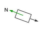
2、up和N差积得到右向量U, U= up X N，归一化U。

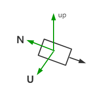
3、然后N和U差积得到垂直于U,N平面的上向量V，V = U x N

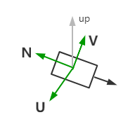
此时我们已经构建好了摄像机坐标系的基向量。也就得到了摄像机坐标系到世界坐标系的过度矩阵R。
$$R=\left[\begin{array}{cccc}U.x& V.x& N.x& 0\\ U.y& V.y& N.y& 0\\ U.z& V.z& N.z& 0\\ 0& 0& 0& 1\end{array}\right]$$
我们的目标是计算世界坐标系中的物体在摄像机坐标系下的坐标，将世界坐标系平移至于相机坐标系重合，此时就可以利用过度矩阵进行坐标变换。
$$T=\left[\begin{array}{cccc}1& 0& 0& camPos.x\\ 0& 1& 0& camPos.y\\ 0& 0& 1& camPos.z\\ 0& 0& 0& 1\end{array}\right]$$

这样这个旋转R和平移T矩阵的组合矩阵M=T∗R，就是将相机坐标系中坐 标变换到世界坐标系中坐标的变换矩阵，那么所求的视图变换矩阵（世界坐标系中坐标转换到相机坐标系中坐标的矩阵）即为这个矩阵的逆：$$view=M^{-1}=(T\ast R{)}^{-1}=R^{-1}\ast T^{-1}$$

$$=\left[\begin{array}{cccc}U.x& U.y& U.z& 0\\ V.x& V.y& V.z& 0\\ N.x& N.y& N.z& 0\\ 0& 0& 0& 1\end{array}\right]\ast \left[\begin{array}{cccc}1& 0& 0& -camPos.x\\ 0& 1& 0& -camPos.y\\ 0& 0& 1& -camPos.z\\ 0& 0& 0& 1\end{array}\right]$$

$$=\left[\begin{array}{cccc}U.x& U.y& U.z& -U\ast camPos\\ V.x& V.y& V.z& -V\ast camPos\\ N.x& N.y& N.z& -N\ast camPos\\ 0& 0& 0& 1\end{array}\right]$$
代码：

Matrix lookat(Vec3f &eye, Vec3f& center, Vec3f& up){
	Vec3f z = (eye - center).normalize();
	Vec3f x = cross(up, z).normalize();
	Vec3f y = cross(z, x).normalize();
	Matrix Minv;
	Minv= Matrix::identity();
	for (int i = 0; i < 3; i++) {
		Minv[0][i] = x[i];
		Minv[1][i] = y[i];
		Minv[2][i] = z[i];
	}
	Minv[0][3] = -1*(x * eye);
	Minv[1][3] = -1*(y * eye);
	Minv[2][3] = -1*(z * eye);

	return Minv;
}

3.投影矩阵

Reference：
OpenGL学习脚印: 投影矩阵和视口变换矩阵(math-projection and viewport matrix)
AirGuanZ：透视投影矩阵推导
YEMI：透视投影矩阵推导
醉里挑灯看剑：投影矩阵推导

投影矩阵主要分为两种，正交投影和透视投影。

两者都会将可见范围（对于透视投影是四棱台，正交投影是长方体）中的点映射到一个立方体中。

透视投影

指定透视投影的视锥需要6个参数，投影平面左边的位置（left），投影平面右边的位置（right），投影平面上边（top）,投影平面下边（bottom）,投影平面距摄像机的距离（near），最远平面距离摄像机的距离（far）。下面会用到这些参数的英文首字母简写。
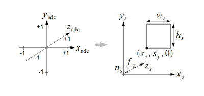
我们的目标是最终将视图坐标(eye)通过投影矩阵变换为裁切坐标(clip)，再通过透视除法将裁切坐标(clip)变成规范化设备坐标系(NDC)坐标，他们的转换关系如下
$$\left[\begin{array}{c}{x}_{chip}\\ y_{chip}\\ z_{chip}\\ w_{chip}\end{array}\right]=P\ast \left[\begin{array}{c}{x}_{eye}\\ y_{eye}\\ z_{eye}\\ w_{eye}\end{array}\right]$$

$$\left[\begin{array}{c}{x}_{ndc}\\ y_{ndc}\\ z_{ndc}\end{array}\right]=\left[\begin{array}{c}{x}_{chip}/w_{chip}\\ y_{chip}/w_{chip}\\ z_{chip}/w_{chip}\end{array}\right]\text{\hspace{1em}(0)}$$
左边是裁切坐标系示意图，右边是ndc示意图

我们假设视锥内有一点$$P(x_{eye},y_{eye},z_{eye})$$

他投影到投影平面的点为$$P(x_{project},y_{project},-near)$$

通过俯视图，我们通过相似三角西得到如下关系

$$\frac{x_{project}}{x_{eye}}=\frac{-near}{z_{eye}}$$

即：
$$x_{project}=\frac{-near\ast x_{eye}}{z_{eye}}\text{\hspace{1em}(1)}$$

同理通过侧视图我们可以得到y的值：
$$y_{project}=\frac{-near\ast y_{eye}}{z_{eye}}\text{\hspace{1em}(2)}$$

因为我们需要Z值保存深度信息后续使用，所以这里先设Z为f(z)，那么我们当前的投影坐标就是：
$$P^{\prime }=(\frac{-near\ast x_{eye}}{z_{eye}},\frac{-near\ast y_{eye}}{z_{eye}},f(z))$$
P’x和P‘y都不是关于Px，Py的线性函数，不能通过矩阵变换得到，我们这里进行等价的齐次变化
$$P^{\prime }=(near\ast x_{eye},near\ast y_{eye},-z_{eye}\ast f(z),-z_{eye})$$

现在我们的运算写成矩阵形式为：
$$\left[\begin{array}{cccc}?& ?& ?& ?\\ ?& ?& ?& ?\\ ?& ?& ?& ?\\ ?& ?& ?& ?\end{array}\right]\ast \left[\begin{array}{c}{x}_{eye}\\ y_{eye}\\ z_{eye}\\ w_{eye}\end{array}\right]=\left[\begin{array}{c}near\ast x_{eye}\\ near\ast y_{eye}\\ f(z)\\ -z_{eye}\end{array}\right]$$
因为 结果的w维已经确定为-Zeye，我们可以推出矩阵最后一行为：
$$\left[\begin{array}{cccc}?& ?& ?& ?\\ ?& ?& ?& ?\\ ?& ?& ?& ?\\ 0& 0& -1& 0\end{array}\right]\ast \left[\begin{array}{c}{x}_{eye}\\ y_{eye}\\ z_{eye}\\ w_{eye}\end{array}\right]=\left[\begin{array}{c}near\ast x_{eye}\\ near\ast y_{eye}\\ f(z)\\ -z_{eye}\end{array}\right]$$
接下来我们将投影平面上的坐标转线性映射到（-1，1）空间。
其中Xp的映射关系如下图所示:

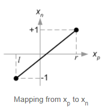
设这条直线方程为
$$X_{ndc}=A\ast X_{project}+B$$
我们已知直线上两点(l,-1), (r,1);
带入直线得：
$$\{\begin{array}{l}-1=A\ast l+B\\ 1=A\ast r+B\end{array}\Rightarrow \{\begin{array}{l}A=\frac{2}{r-l}\\ B=\frac{l+r}{l-r}\end{array}$$

即
$$X_{ndc}=\frac{2}{r-l}\ast X_{project}+\frac{l+r}{l-r}\text{\hspace{1em}(3)}$$

将（1）带入（3）得：
$$X_{ndc}=\frac{2}{r-l}\ast \frac{-near\ast x_{eye}}{z_{eye}}+\frac{l+r}{l-r}$$

同理可得
$$Y_{ndc}=\frac{2}{t-b}\ast \frac{-near\ast y_{eye}}{z_{eye}}+\frac{t+b}{b-t}$$

根据ndc坐标和clip坐标的关系（0）得到
$$X_{clip}=\frac{2\ast n}{r-l}\ast x_{eye}-\frac{l+r}{l-r}\ast z_{eye}$$

$$Y_{clip}=\frac{2\ast n}{t-b}\ast y_{eye}-\frac{t+b}{b-t}\ast z_{eye}$$

由此得到矩阵的前两行为:
$$\left[\begin{array}{cccc}\frac{2\ast n}{r-l}& 0& -\frac{l+r}{l-r}& 0\\ 0& \frac{2\ast n}{t-b}& -\frac{t+b}{b-t}& 0\\ ?& ?& ?& ?\\ 0& 0& -1& 0\end{array}\right]\ast \left[\begin{array}{c}{x}_{eye}\\ y_{eye}\\ z_{eye}\\ w_{eye}\end{array}\right]=\left[\begin{array}{c}{X}_{clip}\\ Y_{clip}\\ f(z)\\ -z_{eye}\end{array}\right]$$
由于Ze投影到平面时结果都为−n，因此寻找zn与之前的x,y分量不太一样。我们知道zn与x,y分量无关，因此上述矩阵P可以书写为：
$$\left[\begin{array}{cccc}\frac{2\ast n}{r-l}& 0& -\frac{l+r}{l-r}& 0\\ 0& \frac{2\ast n}{t-b}& -\frac{t+b}{b-t}& 0\\ 0& 0& A& B\\ 0& 0& -1& 0\end{array}\right]\ast \left[\begin{array}{c}{x}_{eye}\\ y_{eye}\\ z_{eye}\\ w_{eye}\end{array}\right]=\left[\begin{array}{c}{X}_{clip}\\ Y_{clip}\\ f(z)\\ -z_{eye}\end{array}\right]$$
则有
$$Z_{ndc}=\frac{A\ast z_{eye}+B\ast w_{eye}}{-z_{eye}}$$

又因为w_{eye} = 1，故可以化简得：
$$Z_{ndc}=\frac{A\ast z_{eye}+B}{-z_{eye}}\text{\hspace{1em}(4)}$$

我们已知Zndc与Zeye之间的对应关系（-n,-1）（-f，1）带入(4)得：

$$\{\begin{array}{l}-1=\frac{-nA+B}{n}\\ 1=\frac{-fA+B}{f}\end{array}\Rightarrow \{\begin{array}{l}A=-\frac{f+n}{f-n}\\ B=\frac{-2nf}{f-n}\end{array}$$

将AB带入4得到
$$Z_{ndc}=\frac{\frac{-(f+n)}{f-n}\ast z_{eye}+\frac{-2nf}{f-n}}{-z_{eye}}$$

我们的投影矩阵为：
$$\left[\begin{array}{cccc}\frac{2\ast n}{r-l}& 0& -\frac{l+r}{l-r}& 0\\ 0& \frac{2\ast n}{t-b}& -\frac{t+b}{b-t}& 0\\ 0& 0& \frac{-(f+n)}{f-n}& \frac{-2nf}{f-n}\\ 0& 0& -1& 0\end{array}\right]\text{\hspace{1em}(透视投影矩阵)}$$
如果我们的视锥是对称的，满足r = -l，t = -b，则投影矩阵可以化简为
$$\left[\begin{array}{cccc}\frac{n}{r}& 0& 0& 0\\ 0& \frac{n}{t}& 0& 0\\ 0& 0& \frac{-(f+n)}{f-n}& \frac{-2nf}{f-n}\\ 0& 0& -1& 0\end{array}\right]\text{\hspace{1em}(简化的透视投影矩阵)}$$

通过fov计算投影矩阵

另外一种经常使用 的方式是通过视角(Fov)，宽高比(Aspect)来指定透视投影

我们需要给定fov，Aspect，near，far来指定视锥。
通过fov和near，我们可以求得平面高度为
$$\frac{h}{2}=near\ast tan(\frac{\theta }{2})$$
通过平面高度和宽高比，我们可以求得投影平面宽度
$$\frac{w}{2}=\frac{h}{2}\ast aspect=near\ast tan(\frac{\theta }{2})\ast aspect$$

宽高与之前的 l, r, t, b 的对应关系为：
$$\begin{gathered} r=\frac{w}{2}=near\ast tan(\frac{\theta }{2})\ast aspect \\ l=-r \\ t=\frac{h}{2}=near\ast tan(\frac{\theta }{2}) \\ b=-t \end{gathered}$$
带入之前的简化投影矩阵得到
$$\left[\begin{array}{cccc}\frac{1}{tan(\frac{\theta }{2})\ast aspect}& 0& 0& 0\\ 0& \frac{1}{tan(\frac{\theta }{2})}& 0& 0\\ 0& 0& \frac{-(f+n)}{f-n}& \frac{-2nf}{f-n}\\ 0& 0& -1& 0\end{array}\right]\text{\hspace{1em}(fov透视投影矩阵)}$$

Matrix setFrustum(double fovy, double aspect, double near, double far)
{
	double z_range = far - near;
	Matrix matrix;
	matrix= Matrix::identity();
	assert(fovy > 0 && aspect > 0);
	assert(near > 0 && far > 0 && z_range > 0);
	matrix[1][1] = 1 / (float)tan(fovy / 2);
	matrix[0][0] = matrix[1][1] / aspect;
	matrix[2][2] = -(near + far) / z_range;
	matrix[2][3] = -2 * near * far / z_range;
	matrix[3][2] = -1;
	matrix[3][3] = 0;

	return matrix;
}

Zfighting问题

回过头去看透视投影部分，zn与ze的关系式
$$Z_{ndc}=\frac{\frac{-(f+n)}{f-n}\ast z_{eye}+\frac{-2nf}{f-n}}{-z_{eye}}$$
这是一个非线性关系函数，函数关系如图。

从图我们可以看到，在近裁剪平面附近Zn值变化比较大，精确度较好；而在远裁剪平面附近，有一段距离内，Zn近乎持平，精确度不好。当增大远近裁剪平面的范围[−n,−f]后，如右边图所示，我们看到在远裁剪平面附近，不同相机坐标Ze对应的Zn相同，精确度低的现象更为明显，这种深度的精确度引起的问题称之为zFighting。要尽量减小[-n,-f]的范围，以减轻zFighting问题。

正交投影

对于正交投影，有
$$x_p=x_e,y_p=y_e$$

因而可以直接利用Xe与Xn的映射关系：[l,−1],[r,1]，
利用Ye和Yn的映射关系：[b,−1],[t,1]，
以及Ze和Zn的映射关系：[−n,−1],[−f,1]。
与透视矩阵推导类似，我们直接将映射关系[l,−1],[r,1]带入直线。
$$x_{ndc}=A\ast x_{eye}+B$$

解得：
$$x_{ndc}=\frac{2}{r-l}\ast x_{eye}+\frac{r+l}{r-l}$$

同理可以得出
$$y_{ndc}=\frac{2}{t-b}\ast y_{eye}+\frac{t+b}{t-b}$$

$$z_{ndc}=\frac{-2}{f-n}\ast z_{eye}+\frac{f+n}{f-n}$$

对于正交坐标，因为xy维度没有变量z参与，所以可以不进行齐次化。故ndc坐标和裁切坐标相同。我们通过上面三个式子得到正交投影矩阵
$$\left[\begin{array}{cccc}\frac{2}{r-l}& 0& 0& -\frac{r+l}{r-l}\\ 0& \frac{2}{t-b}& 0& -\frac{t+b}{t-b}\\ 0& 0& \frac{-2}{f-n}& -\frac{f+n}{f-n}\\ 0& 0& 0& 1\end{array}\right]\text{\hspace{1em}(正交透视投影矩阵)}$$
如果视锥对称（r = −l, t = −b），我们同样可以进行简化得到：
$$\left[\begin{array}{cccc}\frac{1}{r}& 0& 0& 0\\ 0& \frac{1}{t}& 0& 0\\ 0& 0& \frac{-2}{f-n}& -\frac{f+n}{f-n}\\ 0& 0& 0& 1\end{array}\right]\text{\hspace{1em}(简化正交透视投影矩阵)}$$

4.视窗变换

视窗变换需要指定4个参数，窗口的左下角位置(sx,sy),窗口宽度width，窗口宽度height
在ndc坐标系中，我们的所有坐标范围都在[-1,1]中，视窗变换的目的是让x坐标变换到[sx,sx+width]，y坐标变换到[sy,sy+height]，z坐标变换到[0,1]即：
$$\begin{gathered} x_{screen}=s_x+x(x_{ndc}+1)\ast 0.5\ast width \\ {y}_{screen}=s_y+(y_{ndc}+1)\ast 0.5\ast height \\ {z}_{screen}=(z_{ndc}+1)\ast 0.5 \end{gathered}$$

写为矩阵模式为：
$$\left[\begin{array}{cccc}\frac{width}{2}& 0& 0& s_x+\frac{width}{2}\\ 0& \frac{height}{2}& 0& s_y+\frac{height}{2}\\ 0& 0& \frac{1}{2}& \frac{1}{2}\\ 0& 0& 0& 1\end{array}\right]\text{\hspace{1em}(视口变换矩阵)}$$