时间卷积网络+软阈值+注意力机制实现机械设备剩余寿命预测

1. 关于数据

本模型采用了PHM2012数据竞赛的轴承全寿命数据，以及XJUST-SY轴承全寿命公开数据集进行验证。这两个都是公开数据集，可自行百度/Bing/Google下载，并学习数据文件组织方式。本例仅以PHM2012数据为例，XJUST-SY数据仅需替换数据存储路径，代码不需要变动。

2. 代码非详细解释

2.1 导入必要的库

from keras.layers import Input,concatenate,GRU,Embedding,UpSampling1D,BatchNormalization,Conv1D,MaxPooling1D,Dense,Flatten,Lambda,Dropout,Concatenate,LeakyReLU,BatchNormalization,Reshape,Activation,GlobalAveragePooling1D,AveragePooling1D
from keras import regularizers
from keras.callbacks import EarlyStopping
from keras.optimizers import Adam
from keras.models import Sequential, Model
from keras import backend as K
from keras import Model,regularizers

from scipy import signal
import tensorflow as tf
import numpy as np
import matplotlib.pyplot as plt
from sklearn.model_selection import train_test_split
from sklearn.metrics import mean_squared_error
import xlrd
import os
from sklearn.preprocessing import MinMaxScaler
from keras.models import load_model

import keras
config = tf.ConfigProto()
config.gpu_options.allow_growth = True
keras.backend.tensorflow_backend.set_session(tf.Session(config=config))

import os
os.environ['CUDA_VISIBLE_DEVICES'] = '/gpu:0'

2.2 写函数，导入数据

PHM2010数据Full_Test_Set文件夹下的Bearing1_4数据中，采用了;分隔符将时、分、秒、x向加速度、y向加速度值全都写入一个excel的单元格，与其他几个文件格式不一致，所以写了两个函数，分别用于读取Bearing1_4下数据和其他文件夹下数据。

读取非Bearing1_4数据的函数

#从文件夹里读取水平信号csv数据
def readfile_h(path):
    files = os.listdir(path)
    #将acc文件挑选出来
    files = list(filter(lambda x: x[0:4]=='acc_' , files))
    #解决乱序问题，以第5位到倒数第4位之间的数字的大小排序
    files.sort(key=lambda x:int(x[5:-4]))
   
    rowdata = []
    for file in files:
        info = path+"/"+file
        #将csv文件里的数据转换成矩阵
        data = np.loadtxt(open(info,"rb"), delimiter=',', skiprows=0)
        rowdata = np.hstack((rowdata,data[:,5]))
    return(rowdata)

以下读取非Bearing1_4数据

## 2803个csv文件
train1_1_h = readfile_h('xxxx\Learning_set\Bearing1_1')
#871个csv文件
train1_2_h = readfile_h('xxxx\Learning_set\Bearing1_2')
test1_3_h = readfile_h('xxxx\Full_Test_Set\Bearing1_3')
test1_5_h = readfile_h('xxxx\Full_Test_Set\Bearing1_5')
test1_6_h = readfile_h('xxxx\Full_Test_Set\Bearing1_6')
test1_7_h = readfile_h('xxxx\Full_Test_Set\Bearing1_7')

以下为读取Bearing1_4数据的函数

#读取1_4的数据
def readfile_h(path):
    files = os.listdir(path)
    #将acc文件挑选出来
    files = list(filter(lambda x: x[0:4]=='acc_' , files))
    #解决乱序问题，以第5位到倒数第4位之间的数字的大小排序
    files.sort(key=lambda x:int(x[5:-4]))
   
    rowdata = []
    for file in files:
        info = path+"/"+file
        #将csv文件里的数据转换成矩阵
        data = np.loadtxt(open(info,"rb"), delimiter=';',skiprows=0)
        rowdata = np.hstack((rowdata,data[:,5]))
    return(rowdata)

以下读取Bearing1_4数据

test1_4_h = readfile_h('xxxx\Full_Test_Set\Bearing1_4')

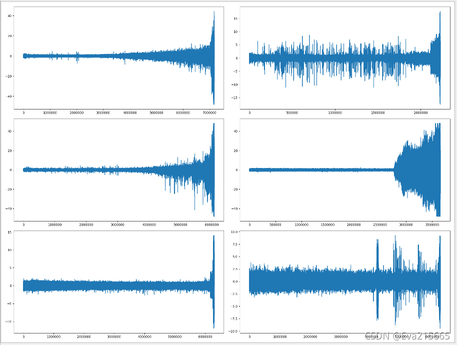
将全寿命数据打印出来看看

plt.figure(figsize=(20,15))
plt.subplot(3, 2, 1)
plt.plot(train1_1_h)
plt.subplot(3, 2, 2)
plt.plot(train1_2_h)
plt.subplot(3, 2, 3)
plt.plot(test1_3_h)
plt.subplot(3, 2, 4)
plt.plot(test1_4_h)
plt.subplot(3, 2, 5)
plt.plot(test1_5_h)
plt.subplot(3, 2, 6)
plt.plot(test1_6_h)
plt.show()

以下为数据标准化，reshape等预处理

#%%
#将数据标准化
mean1_1 =train1_1_h - np.mean(train1_1_h)
train1_h = mean1_1/np.std(train1_1_h)

mean1_2 =train1_2_h - np.mean(train1_2_h)
train2_h =mean1_2/ np.std(train1_2_h)

mean1_3 =test1_3_h - np.mean(test1_3_h)
test3_h = mean1_3/np.std(test1_3_h)

mean1_5 =test1_5_h - np.mean(test1_5_h)
test5_h = mean1_5 /np.std(test1_5_h)

mean1_6 =test1_6_h - np.mean(test1_6_h)
test6_h = mean1_6 /np.std(test1_6_h)

mean1_7=test1_7_h - np.mean(test1_7_h)
test7_h = mean1_7 /np.std(test1_7_h)

mean1_4 =test1_4_h - np.mean(test1_4_h)
test4_h = mean1_4/np.std(test1_4_h)

xtr1_h=train1_h.reshape((-1,2560,1))
xtr2_h=train2_h.reshape((-1,2560,1))
xte3_h= test3_h.reshape(-1,2560,1)
xte4_h= test4_h.reshape(-1,2560,1)
xte5_h = test5_h.reshape(-1,2560,1)
xte6_h = test6_h.reshape(-1,2560,1)
xte7_h = test7_h.reshape(-1,2560,1)
print(xtr1_h.shape)
print(xtr2_h.shape)
print(xte3_h.shape)
print(xte4_h.shape)
print(xte5_h.shape)
print(xte6_h.shape)
print(xte7_h.shape)

以下为写函数并读取y方向的加速度信号，此处其实可以与“读取x方向加速度”的函数进行优化

def readfile_v(path):
    files = os.listdir(path)
    #将acc文件挑选出来
    files = list(filter(lambda x: x[0:4]=='acc_' , files))
    #解决乱序问题，以第5位到倒数第4位之间的数字的大小排序
    files.sort(key=lambda x:int(x[5:-4]))
   
    rowdata = []
    for file in files:
        info = path+"/"+file
        #将csv文件里的数据转换成矩阵
        data = np.loadtxt(open(info,"rb"), delimiter=',',skiprows=0)
        rowdata = np.hstack((rowdata,data[:,4]))
    return(rowdata)

#读取工况1的数据、
#训练数据
#2803个csv文件
train1_1_v = readfile_v('xxxx\Learning_set\Bearing1_1')
#871个csv文件
train1_2_v = readfile_v('xxxx\Learning_set\Bearing1_2')

#测试数据
#test_data 中的2302个文件
test1_3_v = readfile_v('xxxx\Full_Test_Set\Bearing1_3')
test1_5_v = readfile_v('xxxx\Full_Test_Set\Bearing1_5')
test1_6_v = readfile_v('xxxx\Full_Test_Set\Bearing1_6')
test1_7_v = readfile_v('xxxx\Full_Test_Set\Bearing1_7')

#尝试读取1_4的数据
def readfile_v(path):
    files = os.listdir(path)
    #将acc文件挑选出来
    files = list(filter(lambda x: x[0:4]=='acc_' , files))
    #解决乱序问题，以第5位到倒数第4位之间的数字的大小排序
    files.sort(key=lambda x:int(x[5:-4]))
   
    rowdata = []
    for file in files:
        info = path+"/"+file
        #将csv文件里的数据转换成矩阵
        data = np.loadtxt(open(info,"rb"), delimiter=';',skiprows=0)
        rowdata = np.hstack((rowdata,data[:,4]))
    return(rowdata)

test1_4_v = readfile_v('xxxx\Full_Test_Set\Bearing1_4')

将y-方向加速度信号打印出来看看

plt.figure(figsize=(20, 15))
plt.subplot(3, 2, 1)
plt.plot(train1_1_v)
plt.subplot(3, 2, 2)
plt.plot(train1_2_v)
plt.subplot(3, 2, 3)
plt.plot(test1_3_v)
plt.subplot(3, 2, 4)
plt.plot(test1_4_v)
plt.subplot(3, 2, 5)
plt.plot(test1_5_v)
plt.subplot(3, 2, 6)
plt.plot(test1_6_v)
plt.show()

以下为数据标准化、reshape等预处理

#将数据标准化
mean1_1 =train1_1_v - np.mean(train1_1_v)
train1_v = mean1_1/np.std(train1_1_v)

mean1_2 =train1_2_v - np.mean(train1_2_v)
train2_v =mean1_2/ np.std(train1_2_v)


mean1_3 =test1_3_v - np.mean(test1_3_v)
test3_v = mean1_3/np.std(test1_3_v)

mean1_4 =test1_4_v - np.mean(test1_4_v)
test4_v = mean1_4/np.std(test1_4_v)

mean1_5 =test1_5_v - np.mean(test1_5_v)
test5_v = mean1_5 /np.std(test1_5_v)


mean1_6 =test1_6_v - np.mean(test1_6_v)
test6_v = mean1_6 /np.std(test1_6_v)

mean1_7=test1_7_v - np.mean(test1_7_v)
test7_v = mean1_7 /np.std(test1_7_v)

xtr1_v = train1_v.reshape((-1, 2560, 1))
xtr2_v = train2_v.reshape((-1, 2560, 1))
xte3_v = test3_v.reshape((-1, 2560, 1))
xte4_v = test4_v.reshape((-1, 2560, 1))
xte5_v = test5_v.reshape((-1, 2560, 1))
xte6_v = test6_v.reshape((-1, 2560, 1))
xte7_v = test7_v.reshape((-1, 2560, 1))
print(xtr1_v.shape)
print(xtr2_v.shape)
print(xte3_v.shape)
print(xte4_v.shape)
print(xte5_v.shape)
print(xte6_v.shape)
print(xte7_v.shape)

将水平信号与垂直信号拼接起来

#将垂直信号和水平信号拼接在一起
xtr1 = np.hstack((xtr1_v,xtr1_h))
xtr1 = xtr1.reshape((-1,2560,2))
xtr2 = np.hstack((xtr2_v,xtr2_h))
xtr2 = xtr2.reshape((-1,2560,2))
xte3 = np.hstack((xte3_v,xte3_h))
xte3 = xte3.reshape((-1,2560,2))
xte4 = np.hstack((xte4_v,xte4_h))
xte4 = xte4.reshape((-1,2560,2))
xte5 = np.hstack((xte5_v,xte5_h))
xte5 = xte5.reshape((-1,2560,2))
xte6 = np.hstack((xte6_v,xte6_h))
xte6 = xte6.reshape((-1,2560,2))
xte7 = np.hstack((xte7_v,xte7_h))
xte7= xte7.reshape((-1,2560,2))
print(xtr1.shape)
print(xtr2.shape)
print(xte3.shape)
print(xte4.shape)
print(xte5.shape)
print(xte6.shape)
print(xte7.shape)

设置RUL的ground truth

#数据标签，剩余寿命
ytr1 = np.arange(xtr1.shape[0])
ytr1 = ytr1[::-1].reshape((-1,1))
ytr2 = np.arange(xtr2.shape[0])
ytr2 = ytr2[::-1].reshape((-1,1))

yte3 = np.arange(xte3.shape[0])
yte3 = yte3[::-1].reshape((-1,1))

yte4 = np.arange(xte4.shape[0])
yte4 = yte4[::-1].reshape((-1,1))

yte5 = np.arange(xte5.shape[0])
yte5 = yte5[::-1].reshape((-1,1))

yte6 = np.arange(xte6.shape[0])
yte6 = yte6[::-1].reshape((-1,1))

yte7 = np.arange(xte7.shape[0])
yte7 = yte7[::-1].reshape((-1,1))



#将y标签归一化0——1，采用剩余寿命的百分比作为输出标签
#使用剩余寿命的百分比作为标签值
#不乘100为了使用rnn的sigmoid激活函数
min_max_scaler = MinMaxScaler()
ytr1 = min_max_scaler.fit_transform(ytr1)*100
print(ytr1)
ytr2 =  min_max_scaler.fit_transform(ytr2)*100
yte3 =  min_max_scaler.fit_transform(yte3)*100
print(ytr2.shape)
print(yte3.shape)
yte4 =  min_max_scaler.fit_transform(yte4)*100
yte5 =  min_max_scaler.fit_transform(yte5)*100
yte6 =  min_max_scaler.fit_transform(yte6)*100
yte7 =  min_max_scaler.fit_transform(yte7)*100
print(yte4.shape)
print(yte5.shape)
print(yte6.shape)
print(yte7.shape)

数据分组，方便训练与测试

xtr_b1= np.vstack((xtr2,xte3,xte4,xte5,xte6,xte7))
# xtr = xtr.reshape(-1,2560,1)
print(xtr_b1.shape)

ytr_b1 = np.vstack((ytr2,yte3,yte4,yte5,yte6,yte7))
print(ytr_b1.shape)


#将1_2为测试集
xtr_b2= np.vstack((xtr1,xte3,xte4,xte5,xte6,xte7))
print(xtr_b2.shape)

ytr_b2 = np.vstack((ytr1,yte3,yte4,yte5,yte6,yte7))
print(ytr_b2.shape)

#将1_3为测试集
xtr_b3= np.vstack((xtr1,xtr2,xte4,xte5,xte6,xte7))
print(xtr_b3.shape)

ytr_b3 = np.vstack((ytr1,ytr2,yte4,yte5,yte6,yte7))
print(ytr_b3.shape)


#将1_4为测试集
xtr_b4= np.vstack((xtr2,xte3,xte4,xte5,xte6,xte7))
print(xtr_b4.shape)

ytr_b4 = np.vstack((ytr2,yte3,yte4,yte5,yte6,yte7))
print(ytr_b4.shape)

#将1_5为测试集
xtr_b5= np.vstack((xtr1,xtr2,xte3,xte4,xte6,xte7))
print(xtr_b5.shape)

ytr_b5 = np.vstack((ytr1,ytr2,yte3,yte4,yte6,yte7))
print(ytr_b5.shape)


#将1_6为测试集
xtr_b6= np.vstack((xtr1,xtr2,xte3,xte4,xte5,xte7))
print(xtr_b6.shape)

ytr_b6 = np.vstack((ytr1,ytr2,yte3,yte4,yte5,yte7))
print(ytr_b6.shape)

#将1_7为测试集其余做训练集
xtr_b7= np.vstack((xtr1,xtr2,xte3,xte4,xte5,xte6))
print(xtr_b7.shape)

ytr_b7 = np.vstack((ytr1,ytr2,yte3,yte4,yte5,yte6))
print(ytr_b7.shape)

# In[29]:
train_data_list = [(xtr_b1,ytr_b1,xtr1,ytr1),(xtr_b2,ytr_b2,xtr2,ytr2),(xtr_b3,ytr_b3,xte3,yte3),(xtr_b4,ytr_b4,xte4,yte4),(xtr_b5,ytr_b5,xte5,yte5),(xtr_b6,ytr_b6,xte6,yte6),(xtr_b7,ytr_b7,xte7,yte7)]

写了一个评分函数，用于评价除了RMSE, MSE以外的预测性能

#改进后的评分函数
def score(ytr,ypred):
    grade_fr =[]
    grade_be =[]
    Er=ytr-ypred
    n = len(ytr)
    m = n//2
    Er_fr = Er[:m]
    Er_be = Er[m:]
#计算前期得分
    for er in Er_fr:
        if er >0:
            A=np.exp(np.log(0.6)*(er/40))
        else:
            A=np.exp(-np.log(0.6)*(er/10))
        grade_fr.append(A)
    for er in Er_be:
        if er >0:
            A=np.exp(np.log(0.6)*(er/40))
        else:
            A=np.exp(-np.log(0.6)*(er/10))
        grade_be.append(A)
    Score = 0.35*np.mean(grade_fr)+0.65*np.mean(grade_be)
    return Score

以下是核心模型

def abs_backend(inputs):
    return K.abs(inputs)
def  expand_dim_backend(inputs):
    return K.expand_dims(inputs,1)
def sign_backend(inputs):
    return K.sign(inputs)
#换一种残差块
def tcnBlock(incoming,filters,kernel_size,dilation_rate):
    net = incoming
    identity = incoming
    net = BatchNormalization()(net)
#     net = Activation('relu')(net)
    net = keras.layers.LeakyReLU(alpha=0.2)(net)
    net = keras.layers.Dropout(0.3)(net)
    net = Conv1D(filters,kernel_size,padding='causal',dilation_rate=dilation_rate ,kernel_regularizer=regularizers.l2(1e-3))(net)
    net = BatchNormalization()(net)
    net = Activation('relu')(net)
#     net = keras.layers.LeakyReLU(alpha=0.2)(net)
    net = keras.layers.Dropout(0.3)(net)
    net = Conv1D(filters,kernel_size,padding='causal',dilation_rate=dilation_rate, kernel_regularizer=regularizers.l2(1e-3))(net)
    
    #计算全局均值
    net_abs = Lambda(abs_backend)(net)
    abs_mean = GlobalAveragePooling1D()(net_abs)
    #计算系数
    #输出通道数
    scales = Dense(filters, activation=None, kernel_initializer='he_normal', 
                       kernel_regularizer=regularizers.l2(1e-4))(abs_mean)
    scales = BatchNormalization()(scales)
    scales = Activation('relu')(scales)
    scales = Dense(filters, activation='sigmoid', kernel_regularizer=regularizers.l2(1e-4))(scales)
    scales = Lambda(expand_dim_backend)(scales)
   # 计算阈值
    thres = keras.layers.multiply([abs_mean, scales])
    # 软阈值函数
    sub = keras.layers.subtract([net_abs, thres])
    zeros = keras.layers.subtract([sub, sub])
    n_sub = keras.layers.maximum([sub, zeros])
    net = keras.layers.multiply([Lambda(sign_backend)(net), n_sub])
    
    if identity.shape[-1]==filters:
        shortcut=identity
    else:
        shortcut=Conv1D(filters,kernel_size,padding = 'same')(identity)  #shortcut（捷径）
        
    net = keras.layers.add([net,shortcut])
    return net



def build_tcn():
    inputs = Input(shape = (2560,2))
    net = Conv1D(16,12,strides=4,padding='causal',kernel_regularizer=regularizers.l2(1e-3))(inputs)
    net = MaxPooling1D(4)(net)
    net = keras.layers.Dropout(0.4)(net)
    net = tcnBlock(net,12,3,1)
    net = tcnBlock(net,6,3,2)
    net = tcnBlock(net,4,3,4)
    net = GlobalAveragePooling1D()(net)
#     net = keras.layers.Flatten()(net)
#     net = GRU(4,dropout=0.2)(net)
    outputs = Dense(1,activation ='relu')(net)
    model = Model(inputs=inputs, outputs=outputs)
    return model 

以下为后置处理，打印图形，保存数据等

def plot_fig(ytr,y_pred,i,j):
    from matplotlib.ticker import FuncFormatter
    fig, ax = plt.subplots(figsize=(7,5))
    ax.set_title('Bearing B1_'+str(j), fontsize=12)
    ax.set_xlabel('Time(min)', fontsize=12)
    ax.set_ylabel('RUL', fontsize=12)

    #画线
    epochs = range(1,len(y_pred)+1)
    ax.plot(epochs,y_pred,label="Proposed Method")
    ax.plot(epochs,ytr,label="Ground Truth")
    ax.legend(loc=0, numpoints=1)
    #百分比刻度
    def to_percent(temp, position):
        return '%1.0f'%(temp) + '%'
    plt.gca().yaxis.set_major_formatter(FuncFormatter(to_percent))

    # 保存图片
    plt.savefig('xxxxTCN/phm1_'+str(j)+'_'+str(i)+'.png', bbox_inches='tight')


def save_data(yte,y_pred,i,j):
    import pandas as pd
    #将好的曲线数据保存
    plot_data = np.hstack((yte,y_pred))
    dataframe = pd.DataFrame(plot_data)
    dataframe.to_excel('xxxx//TCN//phm1_'+str(j)+'_'+str(i)+'.xls')

def fit_model(xtr,ytr,val_x,val_y):
    model = build_tcn()
    # model.compile(loss='mae', optimizer=Adam(), metrics=['mae'])
    Adam = keras.optimizers.Adam(lr=0.001,beta_1=0.9,beta_2=0.999,epsilon=1e-08)
    model.compile(optimizer=Adam,loss='mse', metrics=['mae'])
    history = model.fit(xtr, ytr, batch_size=128, epochs=800, verbose=1,validation_data = (val_x,val_y))
    return model


def run_model_1(xtr,ytr,xte,yte,i,j):
    model=fit_model(xtr,ytr,xte,yte)
    y_target = model.predict(xtr)
    y_pred = model.predict(xte)
    plot_fig(yte,y_pred,i,j)
    save_data(yte,y_pred,i,j)
    Mae_1 = np.sum(np.absolute(y_pred-yte)/len(yte))
    Rmse_1 = (np.sum((y_pred-yte)**2/len(yte)))**0.5
    Score = score(yte,y_pred)
    return Mae_1,Rmse_1,Score

以下为函数的调用

score_list = []
result = []
train_data = train_data_list[6]
xtr = train_data[0]
print(xtr.shape)
ytr = train_data[1]
xte = train_data[2]
print(xte.shape)
yte = train_data[3]
#%%
Mae, Rmse, Score = run_model_1(xtr, ytr, xte, yte, 0, 1)

使用/改进该代码发表文章时，请引用文章 doi: https://doi.org/10.1016/j.jmsy.2021.07.008