深度学习笔记（9）：第一课第三周作业讲解与代码

最新推荐文章于 2021-04-20 17:07:55 发布

酸菜火锅bb

最新推荐文章于 2021-04-20 17:07:55 发布

阅读量559

点赞数

分类专栏：吴恩达深度学习笔记神经网络笔记

本文链接：https://blog.csdn.net/weixin_43197820/article/details/105474608

版权

笔记同时被 3 个专栏收录

46 篇文章 1 订阅

订阅专栏

吴恩达深度学习笔记

38 篇文章 9 订阅

订阅专栏

神经网络

38 篇文章 3 订阅

订阅专栏

用含有一个隐含层的神经网络分析二维数据

本次任务，我们要建立一个浅层的神经网络，具体实现一下正向传播，反向传播，梯度下降，和模型预测可视化的实践过程。

首先查清楚一共有多少个训练实例

我们要通过获取变量的维度来得到各个数据。代码如下：

### START CODE HERE ### (≈ 3 lines of code)
shape_X = X.shape
shape_Y = Y.shape
m = shape_X[1]  
#Size of the train set
### END CODE HERE ###

print ('The shape of X is: ' + str(shape_X))
print ('The shape of Y is: ' + str(shape_Y))
print ('I have m = %d training examples!' % (m))

神经网络模型的总纲领

从上面我们可以得知Logistic回归不适用于“flower数据集”。现在你将训练带有单个隐藏层的神经网络。

这是我们的模型：

Image Name

数学原理：

例如 $x^{(i)}$ :
$z^{[1] (i)} = W^{[1]} x^{(i)} + b^{[1] (i)}\tag{1}$
$a^{[1] (i)} = \tanh(z^{[1] (i)})\tag{2}$
$z^{[2] (i)} = W^{[2]} a^{[1] (i)} + b^{[2] (i)}\tag{3}$
$\hat{y}^{(i)} = a^{[2] (i)} = \sigma(z^{ [2] (i)})\tag{4}$
$KaTeX parse error: Undefined control sequence: \mbox at position 43: …gin{cases} 1 & \̲m̲b̲o̲x̲{if } a^{[2](i)…$

根据所有的预测数据，你还可以如下计算损失 $J$ :
$\frac{1}{m} \sum\limits_{i = 0}^{m} \large\left(\small y^{(i)}\log\left(a^{[2] (i)}\right) + (1-y^{(i)})\log\left(1- a^{[2] (i)}\right) \large \right) \small \tag{6}$

提示：
建立神经网络的一般方法是：
1.定义神经网络结构（输入单元数，隐藏单元数等）。
2.初始化模型的参数
3.循环：

实现前向传播
计算损失
后向传播以获得梯度
更新参数（梯度下降）

我们通常会构建辅助函数来计算第1-3步，然后将它们合并为nn_model()函数。一旦构建了nn_model()并学习了正确的参数，就可以对新数据进行预测。

定义神经网络结构

# GRADED FUNCTION: layer_sizes

def layer_sizes(X, Y):
    """
    Arguments:
    X -- input dataset of shape (input size, number of examples)
    Y -- labels of shape (output size, number of examples)
    
    Returns:
    n_x -- the size of the input layer
    n_h -- the size of the hidden layer
    n_y -- the size of the output layer
    """
    ### START CODE HERE ### (≈ 3 lines of code)
    n_x=X.shape[0]
    n_h=4
    n_y=Y.shape[0]
    ### END CODE HERE ###
    return (n_x, n_h, n_y)

初始化模型参数

用randn随机生成 $w$ 矩阵初始向量，用zeros生成 $b$ 初始向量

# GRADED FUNCTION: initialize_parameters

def initialize_parameters(n_x, n_h, n_y):
    """
    Argument:
    n_x -- size of the input layer
    n_h -- size of the hidden layer
    n_y -- size of the output layer
    
    Returns:
    params -- python dictionary containing your parameters:
                    W1 -- weight matrix of shape (n_h, n_x)
                    b1 -- bias vector of shape (n_h, 1)
                    W2 -- weight matrix of shape (n_y, n_h)
                    b2 -- bias vector of shape (n_y, 1)
    """
    
    np.random.seed(2) # we set up a seed so that your output matches ours although the initialization is random.
    
    ### START CODE HERE ### (≈ 4 lines of code)
    W1 = np.random.randn(n_h,n_x)*0.01
    b1 = np.zeros((n_h,1))
    W2 = np.random.randn(n_y,n_h)*0.01
    b2 = np.zeros((n_y,1))
    ### END CODE HERE ###
    
    assert (W1.shape == (n_h, n_x))
    assert (b1.shape == (n_h, 1))
    assert (W2.shape == (n_y, n_h))
    assert (b2.shape == (n_y, 1))
    
    parameters = {"W1": W1,
                  "b1": b1,
                  "W2": W2,
                  "b2": b2}
    
    return parameters

循环

正向传播，将X到Z到A到Z到A

# GRADED FUNCTION: forward_propagation

def forward_propagation(X, parameters):
    """
    Argument:
    X -- input data of size (n_x, m)
    parameters -- python dictionary containing your parameters (output of initialization function)
    
    Returns:
    A2 -- The sigmoid output of the second activation
    cache -- a dictionary containing "Z1", "A1", "Z2" and "A2"
    """
    # Retrieve each parameter from the dictionary "parameters"
    ### START CODE HERE ### (≈ 4 lines of code)
    W1=parameters['W1']
    W2=parameters['W2']
    b1=parameters['b1']
    b2=parameters['b2']
    ### END CODE HERE ###
    
    # Implement Forward Propagation to calculate A2 (probabilities)
    ### START CODE HERE ### (≈ 4 lines of code)
    Z1 = np.dot(W1,X)+b1
    A1 = np.tanh(Z1)
    Z2 = np.dot(W2,A1)+b2
    A2 = sigmoid(Z2)
    ### END CODE HERE ###
    
    assert(A2.shape == (1, X.shape[1]))
    
    cache = {"Z1": Z1,
             "A1": A1,
             "Z2": Z2,
             "A2": A2}
    
    return A2, cache

计算损失

公式套用好即可，这里面内积使用mutiply，然后别忘记除以m

# GRADED FUNCTION: compute_cost

def compute_cost(A2, Y, parameters):
    """
    Computes the cross-entropy cost given in equation (13)
    
    Arguments:
    A2 -- The sigmoid output of the second activation, of shape (1, number of examples)
    Y -- "true" labels vector of shape (1, number of examples)
    parameters -- python dictionary containing your parameters W1, b1, W2 and b2
    
    Returns:
    cost -- cross-entropy cost given equation (13)
    """
    
    m = Y.shape[1] # number of example

    # Compute the cross-entropy cost
    ### START CODE HERE ### (≈ 2 lines of code)
     
    logprobs = np.multiply(np.log(A2),Y)
    cost = - np.sum(logprobs)
    logprobs = np.multiply(np.log(1-A2),1-Y)
    cost = cost - np.sum(logprobs)
    cost = cost /m
    
    ### END CODE HERE ###
    
    cost = np.squeeze(cost)     # makes sure cost is the dimension we expect. 
                                # E.g., turns [[17]] into 17 
    assert(isinstance(cost, float))
    
    return cost

现在，通过使用在正向传播期间计算的缓存，你可以实现后向传播。

标题实现函数`backward_propagation（）`。

说明：
反向传播通常是深度学习中最难（最数学）的部分。为了帮助你更好地了解，我们提供了反向传播课程的幻灯片。你将要使用此幻灯片右侧的六个方程式以构建向量化实现。（所涉及到的公式，我已经在上一篇博文中详细推导过了，这一部分就严格按照其实现就好了）

Image Name

$\frac{\partial \mathcal{J} }{ \partial z_{2}^{(i)} } = \frac{1}{m} (a^{[2](i)} - y^{(i)})$

$\frac{\partial \mathcal{J} }{ \partial W_2 } = \frac{\partial \mathcal{J} }{ \partial z_{2}^{(i)}} a^{[1](i)T}$

$\frac{\partial \mathcal{J} }{ \partial b_2 } = \sum_i{\frac{\partial \mathcal{J} }{ \partial z_{2}^{(i)}}}$

$\frac{\partial \mathcal{J} }{ \partial z_{1}^{(i)} } = W_2^T \frac{\partial \mathcal{J} }{ \partial z_{2}^{(i)} } * ( 1 - a^{[1](i)2})$

$\frac{\partial \mathcal{J} }{ \partial W_1 } = \frac{\partial \mathcal{J} }{ \partial z_{1}^{(i)}} X^T$

$\frac{\partial \mathcal{J} _i }{ \partial b_1 } = \sum_i{\frac{\partial \mathcal{J} }{ \partial z_{1}^{(i)}}}$

请注意， $*$ 表示元素乘法。
你将使用在深度学习中很常见的编码表示方法：
- dW1 = $\frac{\partial \mathcal{J} }{ \partial W_1 }$
- db1 = $\frac{\partial \mathcal{J} }{ \partial b_1 }$
- dW2 = $\frac{\partial \mathcal{J} }{ \partial W_2 }$
- db2 = $\frac{\partial \mathcal{J} }{ \partial b_2 }$
提示：
-要计算dZ1，你首先需要计算 $g^{[1]'}(Z^{[1]})$ 。由于 $g^{[1]}(.)$ 是tanh激活函数，因此如果 $a = g^{[1]}(z)$ 则 $g^{[1]'}(z) = 1-a^2$ 。所以你可以使用(1 - np.power(A1, 2))计算 $g^{[1]'}(Z^{[1]})$ 。
代码如下：

# GRADED FUNCTION: backward_propagation

def backward_propagation(parameters, cache, X, Y):
    """
    Implement the backward propagation using the instructions above.
    
    Arguments:
    parameters -- python dictionary containing our parameters 
    cache -- a dictionary containing "Z1", "A1", "Z2" and "A2".
    X -- input data of shape (2, number of examples)
    Y -- "true" labels vector of shape (1, number of examples)
    
    Returns:
    grads -- python dictionary containing your gradients with respect to different parameters
    """
    m = X.shape[1]
    
    # First, retrieve W1 and W2 from the dictionary "parameters".
    ### START CODE HERE ### (≈ 2 lines of code)
    W1 = parameters['W1']
    W2 = parameters['W2']
    ### END CODE HERE ###
        
    # Retrieve also A1 and A2 from dictionary "cache".
    ### START CODE HERE ### (≈ 2 lines of code)
    A1 = cache['A1']
    A2 = cache['A2']
    ### END CODE HERE ###
    
    # Backward propagation: calculate dW1, db1, dW2, db2. 
    ### START CODE HERE ### (≈ 6 lines of code, corresponding to 6 equations on slide above)
    dZ2 = A2 - Y
    dW2 = 1/m*(np.dot(dZ2,A1.T))
    db2 = 1/m*np.sum(dZ2,axis = 1,keepdims = True)
    
    dZ1 = np.dot(W2.T,dZ2)*(1 - np.power(A1, 2))
    dW1 = 1/m*(np.dot(dZ1,X.T))
    db1 = 1/m*np.sum(dZ1,axis = 1,keepdims = True)
   
   
    ### END CODE HERE ###
    
    grads = {"dW1": dW1,
             "db1": db1,
             "dW2": dW2,
             "db2": db2}
    
    return grads

良好不良好学习率的梯度下降效果·

Image Name

梯度下降参数更新

代码如下

# GRADED FUNCTION: update_parameters

def update_parameters(parameters, grads, learning_rate = 1.2):
    """
    Updates parameters using the gradient descent update rule given above
    
    Arguments:
    parameters -- python dictionary containing your parameters 
    grads -- python dictionary containing your gradients 
    
    Returns:
    parameters -- python dictionary containing your updated parameters 
    """
    # Retrieve each parameter from the dictionary "parameters"
    ### START CODE HERE ### (≈ 4 lines of code)
    W1 = parameters['W1']
    b1 = parameters['b1']
    W2 = parameters['W2']
    b2 = parameters['b2']
    ### END CODE HERE ###
    
    # Retrieve each gradient from the dictionary "grads"
    ### START CODE HERE ### (≈ 4 lines of code)
    dW1 = grads['dW1']
    dW2 = grads['dW2']
    db1 = grads['db1']
    db2 = grads['db2']
    ## END CODE HERE ###
    
    
    # Update rule for each parameter
    ### START CODE HERE ### (≈ 4 lines of code)
    W1=W1-learning_rate*dW1
    W2=W2-learning_rate*dW2
    b1=b1-learning_rate*db1
    b2=b2-learning_rate*db2
    ### END CODE HERE ###
    
    parameters = {"W1": W1,
                  "b1": b1,
                  "W2": W2,
                  "b2": b2}
    
    return parameters

用正确的顺序将前面所实现的函数组合成`nn_model`

注释里面说的很明白了，不犯浑就好

# GRADED FUNCTION: nn_model

def nn_model(X, Y, n_h, num_iterations = 10000, print_cost=False):
    """
    Arguments:
    X -- dataset of shape (2, number of examples)
    Y -- labels of shape (1, number of examples)
    n_h -- size of the hidden layer
    num_iterations -- Number of iterations in gradient descent loop
    print_cost -- if True, print the cost every 1000 iterations
    
    Returns:
    parameters -- parameters learnt by the model. They can then be used to predict.
    """
    
    np.random.seed(3)
    n_x = layer_sizes(X, Y)[0]
    n_y = layer_sizes(X, Y)[2]
    
    # Initialize parameters, then retrieve W1, b1, W2, b2. Inputs: "n_x, n_h, n_y". Outputs = "W1, b1, W2, b2, parameters".
    ### START CODE HERE ### (≈ 5 lines of code)
    parameters = initialize_parameters(n_x, n_h, n_y)
    W1 = parameters['W1']
    W2 = parameters['W2']
    b1 = parameters['b1']
    b2 = parameters['b2']
    ### END CODE HERE ###
    
    # Loop (gradient descent)

    for i in range(0, num_iterations):
         
        ### START CODE HERE ### (≈ 4 lines of code)
        # Forward propagation. Inputs: "X, parameters". Outputs: "A2, cache".
        A2, cache = forward_propagation(X, parameters)
        
        # Cost function. Inputs: "A2, Y, parameters". Outputs: "cost".
        cost = compute_cost(A2, Y, parameters)
 
        # Backpropagation. Inputs: "parameters, cache, X, Y". Outputs: "grads".
        grads = backward_propagation(parameters, cache, X, Y)
 
        # Gradient descent parameter update. Inputs: "parameters, grads". Outputs: "parameters".
        parameters = update_parameters(parameters, grads)
        
        ### END CODE HERE ###
        
        # Print the cost every 1000 iterations
        if print_cost and i % 1000 == 0:
            print ("Cost after iteration %i: %f" %(i, cost))

    return parameters

预测

这里面用了一个小trick对于np.array整体做判断可以生成一个array数组,如X_new = (X > threshold)

# GRADED FUNCTION: predict

def predict(parameters, X):
    """
    Using the learned parameters, predicts a class for each example in X
    
    Arguments:
    parameters -- python dictionary containing your parameters 
    X -- input data of size (n_x, m)
    
    Returns
    predictions -- vector of predictions of our model (red: 0 / blue: 1)
    """
    
    # Computes probabilities using forward propagation, and classifies to 0/1 using 0.5 as the threshold.
  ### START CODE HERE ### (≈ 2 lines of code)
    A2,cache = forward_propagation(X, parameters)
    predictions = (np.abs(A2) > 0.5)
    ### END CODE HERE ###
    
    return predictions

不同隐含层所对应的不同的效果

的确隐含层越高表达力越强，但最后的情况可以说正在向过拟合逼近
在这里插入图片描述

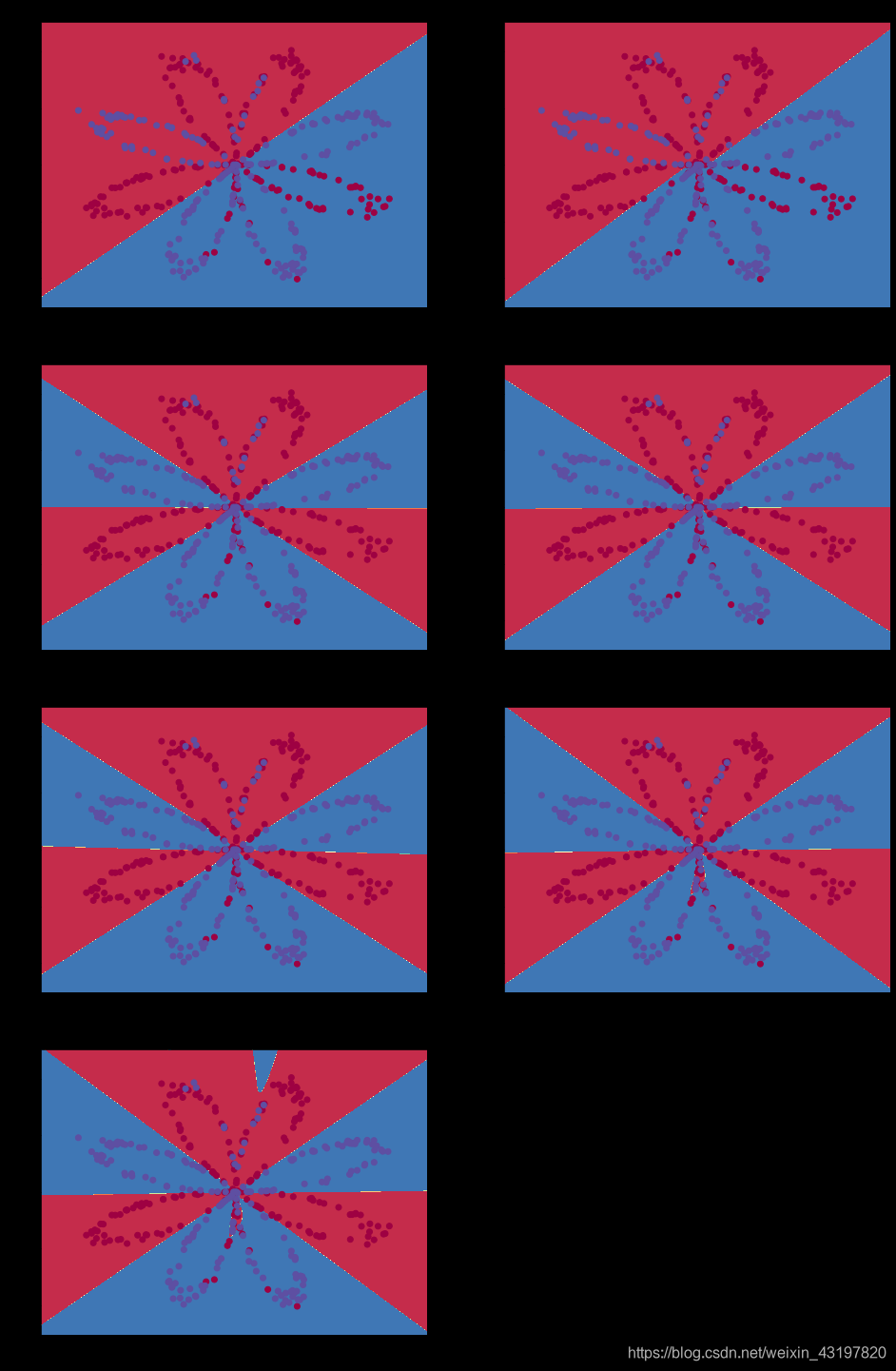
测试在其他测试集的性能

我们只需要加载不同的dataset去尝试就可以
先运行下图
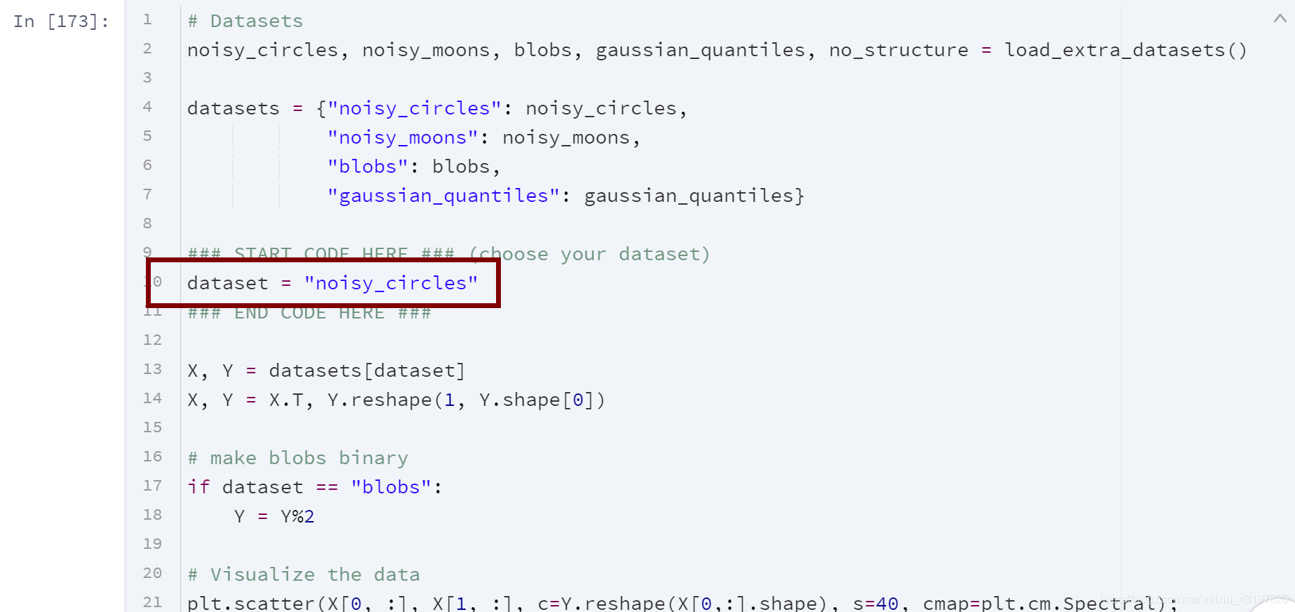在这里插入图片描述再下图

完

酸菜火锅bb

关注

0
点赞
踩
0

收藏

觉得还不错? 一键收藏
0
评论
深度学习笔记（9）：第一课第三周作业讲解与代码

用含有一个隐含层的神经网络分析二维数据本次任务，我们要建立一个浅层的神经网络，具体实现一下正向传播，反向传播，梯度下降，和模型预测可视化的实践过程。首先查清楚一共有多少个训练实例我们要通过获取变量的维度来得到各个数据。代码如下：### START CODE HERE ### (≈ 3 lines of code)shape_X = X.shapeshape_Y = Y.shapem ...
复制链接

扫一扫