


>- **🍨 本文为[🔗365天深度学习训练营]中的学习记录博客**
>- **🍖 原作者:[K同学啊]**
本人往期文章可查阅: 深度学习总结
一、前期工作
本文将采用CNN实现多云、下雨、晴、日出四种天气状态的识别。较上篇文章,本文为了增加模型的泛化能力,新增了Dropout层并且将最大池化层调整成了平均池化层。
🦾我的环境:
- 语言环境:Python3.11.7
- 编译器:jupyter notebook
- 深度学习环境:TensorFlow2.13.0
1. 设置GPU
如果使用的是CPU可以忽略这步
import tensorflow as tf

gpus=tf.config.list_physical_devices("GPU")

if gpus:
    gpu0=gpus[0]  #如果有多个GPU,仅使用第0个GPU
    tf.config.experimental.set_memory_growth(gpu0,True) #设置GPU显存用量按需使用
    tf.config.set_visible_devices([gpu0],"GPU")
2. 导入数据
import pathlib

data_dir="D:\THE MNIST DATABASE\weather_photos"
data_dir=pathlib.Path(data_dir)
3. 查看数据
数据集一共分为cloudy、rain、shine、sunrise四类,分别存放于weather_photos文件夹中以各自名字命名的子文件夹中。
image_count=len(list(data_dir.glob('*/*.jpg')))

print("图片总数为:",image_count)
运行结果:
图片总数为: 1125import PIL
roses=list(data_dir.glob('sunrise/*.jpg'))
PIL.Image.open(str(roses[0]))运行结果:

二、数据预处理
1. 加载数据
使用image_dataset_from_directory方法将磁盘中的数据加载到tf.data.Dataset中。
函数原型:
tf.keras.preprocessing.image_dataset_from_directory(
directory,
labels="inferred",
label_mode="int",
class_names=None,
color_mode="rgb",
batch_size=32,
image_size=(256, 256),
shuffle=True,
seed=None,
validation_split=None,
subset=None,
interpolation="bilinear",
follow_links=False,
)
参数
directory: 数据所在目录。如果标签是inferred(默认),则它应该包含子目录,每个目录包含一个类的图像。否则,将忽略目录结构。
labels: inferred(标签从目录结构生成),或者是整数标签的列表/元组,其大小与目录中找到的图像文件的数量相同。标签应根据图像文件路径的字母顺序排序(通过Python中的os.walk(directory)获得)。
label_mode:标签将被编码为分类向量(使用的损失函数应为:categorical_crossentropy loss).
int:标签将被编码成整数(使用的损失函数应为:sparse_categorical_crossentropy loss)。
categorical:标签将被编码为分类向量(使用的损失函数应为:categorical_crossentropy loss)。
binary:意味着标签(只能有2个)被编码为值为0或1的float32标量(例如:binary_crossentropy)。
None:(无标签)。
class_names: 仅当labels为inferred时有效。这是类名称的明确列表(必须与子目录的名称匹配)。用于控制类的顺序(否则使用字母数字顺序)。
color_mode: grayscale、rgb、rgba之一。默认值:rgb。图像将被转换为1、3或者4通道。
batch_size: 数据批次的大小。默认值:32
image_size: 从磁盘读取数据后将其重新调整大小。默认:(256,256)。由于管道处理的图像批次必须具有相同的大小,因此该参数必须提供。
shuffle: 是否打乱数据。默认值:True。如果设置为False,则按字母数字顺序对数据进行排序。
seed: 用于shuffle和转换的可选随机种子。
validation_split: 0和1之间的可选浮点数,可保留一部分数据用于验证。
subset: training或validation之一。仅在设置validation_split时使用。
interpolation: 字符串,当调整图像大小时使用的插值方法。默认为:bilinear。支持bilinear, nearest, bicubic, area, lanczos3, lanczos5, gaussian, mitchellcubic。
follow_links: 是否访问符号链接指向的子目录。默认:False。
建立训练集:
batch_size=32
img_height=180
img_width=180

train_ds=tf.keras.preprocessing.image_dataset_from_directory(
    data_dir,
    validation_split=0.2,
    subset="training",
    seed=123,
    image_size=(img_height,img_width),
    batch_size=batch_size
)
运行结果:
Found 1125 files belonging to 4 classes.
Using 900 files for training.
建立测试集:
val_ds=tf.keras.preprocessing.image_dataset_from_directory(
    data_dir,
    validation_split=0.2,
    subset="validation",
    seed=123,
    image_size=(img_height,img_width),
    batch_size=batch_size
)
运行结果:
Found 1125 files belonging to 4 classes.
Using 225 files for validation.
我们可以通过class_names输出数据集的标签。标签将按字母顺序对应于目录名称。
class_names=train_ds.class_names
print(class_names)
运行结果:
['cloudy', 'rain', 'shine', 'sunrise']2. 可视化数据
import matplotlib.pyplot as plt

plt.figure(figsize=(20,10))

for images,labels in train_ds.take(1):
    for i in range(20):
        ax=plt.subplot(5,10,i+1)

        plt.imshow(images[i].numpy().astype("uint8"))
        plt.title(class_names[labels[i]])

        plt.axis("off")
运行结果:

3. 再次检查数据
for image_batch,labels_batch in train_ds:
    print(image_batch.shape)
    print(labels_batch.shape)
    break
运行结果:
(32, 180, 180, 3)
(32,)Image_batch是形状的张量(32,180,180,3)。这是一批形状180x180x3的32张图片(最后一维指的是彩色通道RGB)。
Label_batch是形状(32,)的张量,这些标签对应32张图片
4. 配置数据集
- shuffle():打乱数据,关于此函数的详细介绍可以参考:https://zhuanlan.zhihu.com/p/42417456
- prefetch():预取数据,加速运行
prefetch()功能详细介绍:CPU 正在准备数据时,加速器处于空闲状态。相反,当加速器正在训练模型时,CPU 处于空闲状态。因此,训练所用的时间是 CPU 预处理时间和加速器训练时间的总和。prefetch()将训练步骤的预处理和模型执行过程重叠到一起。当加速器正在执行第 N 个训练步时,CPU 正在准备第 N+1 步的数据。这样做不仅可以最大限度地缩短训练的单步用时(而不是总用时),而且可以缩短提取和转换数据所需的时间。如果不使用prefetch(),CPU 和 GPU/TPU 在大部分时间都处于空闲状态:

使用prefetch()可显著减少空闲时间:

- cache():将数据集缓存到内存当中,加速运行
AUTOTUNE=tf.data.AUTOTUNE

train_ds=train_ds.cache().shuffle(1000).prefetch(buffer_size=AUTOTUNE)
val_ds=val_ds.cache().prefetch(buffer_size=AUTOTUNE)
三、构建CNN网络
卷积神经网络(CNN)的输入是张量 (Tensor) 形式的 (image_height, image_width, color_channels),包含了图像高度、宽度及颜色信息。不需要输入batch size。color_channels 为 (R,G,B) 分别对应 RGB 的三个颜色通道(color channel)。在此示例中,我们的 CNN 输入形状是 (180, 180, 3)。我们需要在声明第一层时将形状赋值给参数input_shape。
网络结构图(可单击放大查看):
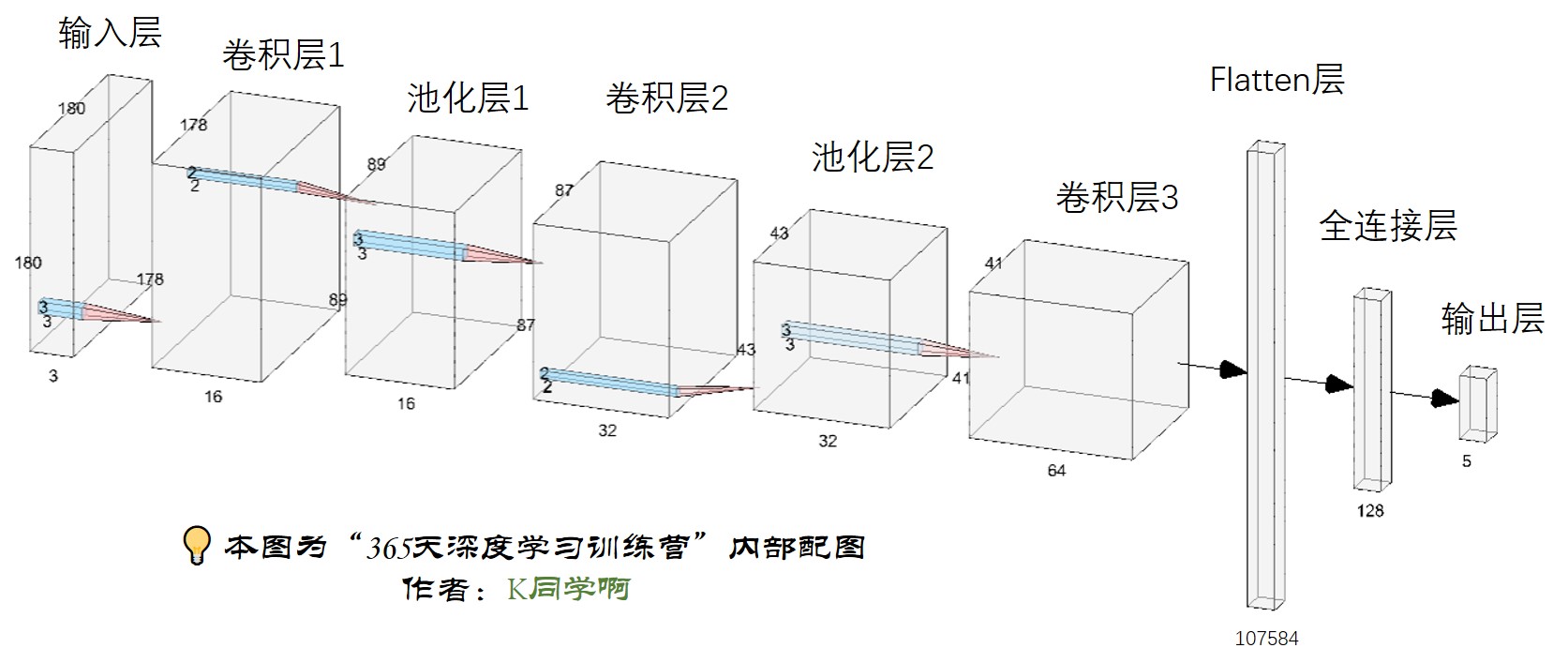
from tensorflow.keras import models,layers
num_classes=4

model=models.Sequential([
    layers.experimental.preprocessing.Rescaling(1./255,input_shape=(img_height,img_width,3)),#卷积层1,卷积核3*3

    layers.Conv2D(16,(3,3),activation='relu',input_shape=(img_height,img_width,3)),
    layers.AveragePooling2D((2,2)),  #池化层1,2*2采样
    layers.Conv2D(32,(3,3),activation='relu'),  #卷积层2,卷积核3*3
    layers.AveragePooling2D((2,2)),  #池化层2,2*2采样
    layers.Conv2D(64,(3,3),activation='relu'),  #卷积层3,卷积核3*3
    layers.Dropout(0.3),

    layers.Flatten(),  #Flatten层,连接卷积层与全连接层
    layers.Dense(128,activation='relu'), #全连接层,特征进一步提取
    layers.Dense(num_classes)  #输出层,输出预期结果
])

model.summary() #打印网络结构
运行结果:
Model: "sequential_1"
_________________________________________________________________
 Layer (type)                Output Shape              Param #
=================================================================
 rescaling (Rescaling)       (None, 180, 180, 3)       0

 conv2d (Conv2D)             (None, 178, 178, 16)      448

 average_pooling2d (Average  (None, 89, 89, 16)        0
 Pooling2D)

 conv2d_1 (Conv2D)           (None, 87, 87, 32)        4640

 average_pooling2d_1 (Avera  (None, 43, 43, 32)        0
 gePooling2D)

 conv2d_2 (Conv2D)           (None, 41, 41, 64)        18496

 dropout (Dropout)           (None, 41, 41, 64)        0

 flatten (Flatten)           (None, 107584)            0

 dense (Dense)               (None, 128)               13770880

 dense_1 (Dense)             (None, 4)                 516

=================================================================
Total params: 13794980 (52.62 MB)
Trainable params: 13794980 (52.62 MB)
Non-trainable params: 0 (0.00 Byte)
_________________________________________________________________
四、编译
在准备对模型进行训练之前,还需要再对其进行一些设置。以下内容是在模型的编译步骤中添加的:
- 损失函数(loss):用于衡量模型在训练期间的准确率。
- 优化器(optimizer):决定模型如何根据其看到的数据和自身的损失函数进行更新。
- 指标(metrics):用于监控训练和测试步骤。以下示例使用了准确率,即被正确分类的图像的比率。
#设置优化器
opt=tf.keras.optimizers.Adam(learning_rate=0.001)

model.compile(optimizer=opt,
              loss=tf.keras.losses.SparseCategoricalCrossentropy(from_logits=True),
              metrics=['accuracy'])
五、训练模型
epochs=10

history=model.fit(
    train_ds,
    validation_data=val_ds,
    epochs=epochs
)
运行结果:
Epoch 1/10
29/29 [==============================] - 23s 576ms/step - loss: 0.9197 - accuracy: 0.6456 - val_loss: 0.6145 - val_accuracy: 0.7511
Epoch 2/10
29/29 [==============================] - 14s 476ms/step - loss: 0.4821 - accuracy: 0.8300 - val_loss: 0.4696 - val_accuracy: 0.8044
Epoch 3/10
29/29 [==============================] - 14s 467ms/step - loss: 0.3109 - accuracy: 0.8811 - val_loss: 0.4615 - val_accuracy: 0.8400
Epoch 4/10
29/29 [==============================] - 14s 494ms/step - loss: 0.2540 - accuracy: 0.9078 - val_loss: 0.4305 - val_accuracy: 0.8267
Epoch 5/10
29/29 [==============================] - 13s 465ms/step - loss: 0.1992 - accuracy: 0.9256 - val_loss: 0.4801 - val_accuracy: 0.8356
Epoch 6/10
29/29 [==============================] - 13s 460ms/step - loss: 0.1609 - accuracy: 0.9400 - val_loss: 0.3793 - val_accuracy: 0.8711
Epoch 7/10
29/29 [==============================] - 13s 446ms/step - loss: 0.1039 - accuracy: 0.9656 - val_loss: 0.4324 - val_accuracy: 0.8533
Epoch 8/10
29/29 [==============================] - 13s 464ms/step - loss: 0.2382 - accuracy: 0.9122 - val_loss: 0.4929 - val_accuracy: 0.8178
Epoch 9/10
29/29 [==============================] - 13s 456ms/step - loss: 0.1779 - accuracy: 0.9256 - val_loss: 0.6137 - val_accuracy: 0.8000
Epoch 10/10
29/29 [==============================] - 13s 458ms/step - loss: 0.1023 - accuracy: 0.9678 - val_loss: 0.4647 - val_accuracy: 0.8533
六、模型评估
acc=history.history['accuracy']
val_acc=history.history['val_accuracy']

loss=history.history['loss']
val_loss=history.history['val_loss']

epochs_range=range(epochs)

plt.figure(figsize=(12,4))
plt.subplot(1,2,1)
plt.plot(epochs_range,acc,label='Training Accuracy')
plt.plot(epochs_range,val_acc,label='Validation Accuracy')
plt.legend(loc='lower right')
plt.title('Training and Validation Accuracy')

plt.subplot(1,2,2)
plt.plot(epochs_range,loss,label='Training Loss')
plt.plot(epochs_range,val_loss,label='Validation Loss')
plt.legend(loc='upper right')
plt.title('Training and Validation Loss')
plt.show()
运行结果:

七、心得体会
本周项目在运行过程中,添加了正则化方法,有效防止了模型出现过拟合现象。


 被折叠的 条评论
为什么被折叠?
被折叠的 条评论
为什么被折叠?
 到【灌水乐园】发言


