吴恩达深度学习 5.2 序列模型-NLP和词嵌入

1. 知识点

• 单词的向量表示：

        one-hot：向量长度为词典全部单词数，对应单词的位置用1表示，其他位置用0表示。缺点是每两个单词向量的乘积都为0，无法获取词与词之彰的相似性和相关性。        

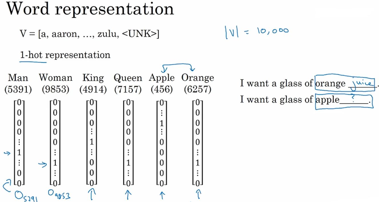
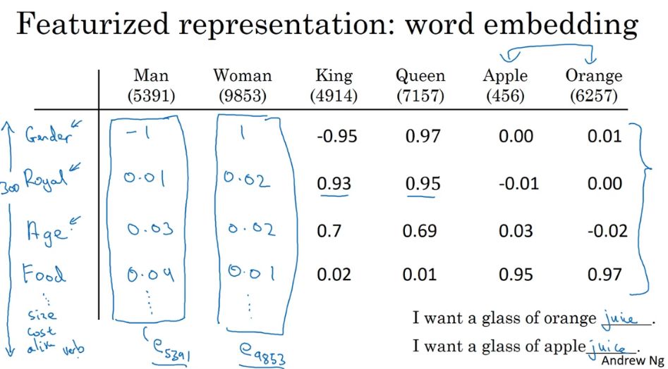
        词嵌入：用不同特征对各个词汇进行表征，相对与不同的特征，不同的单词均有不同的值。

• 词嵌入的应用

        名字实体识别：比如，数据集不包含durain（榴莲）词汇，无法对包含durain的句子做实体识别。但我们从durain的词嵌入向量中获得durain是一种水果，这就有助于对句子中的durain进行名字实体识别。

        迁移学习：利用训练好的词嵌入模型，迁移到训练数据集较小的新任务上，再使用新的标记数据 对词嵌入模型进行微调。

        

• 词嵌入的特性

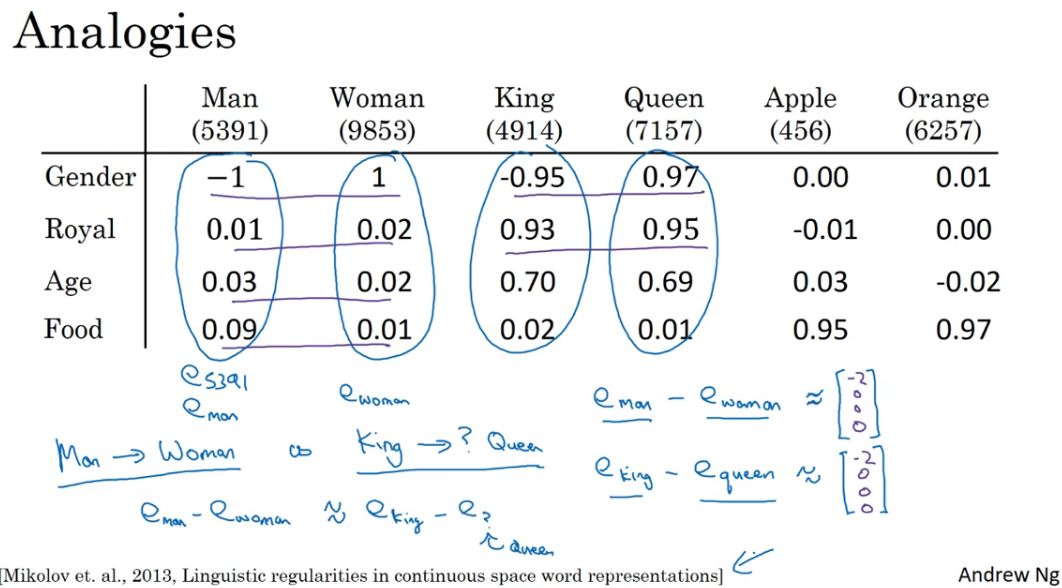
        类比推理特性：比如，man-woman之间的距离，接近king-queen之间的距离，这两对单词之间是类比关系。

        相似度函数：衡量词嵌入向量的相似度函数有余弦相似度、欧氏距离等

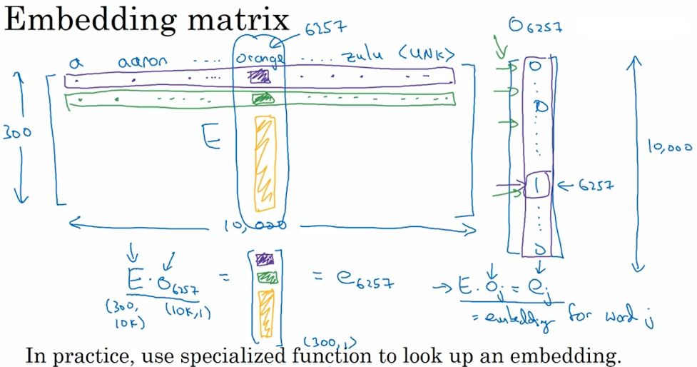
• 嵌入矩阵：

• 词嵌入的学习 

        早期的学习：将嵌入矩阵作为输入，标签为单词。用softmax()激活。

        对目标词的上下文进行选择：根据不同的总是，选择对目标词影响较大的上下文，比如目标词之前几个词、目标词前后几个词、目前词前面一个词、目前词附近一个词。

• Word2Vec词嵌入算法

        1）选择上下文C和目标词T；

        2）用C的词嵌入向量作为输入，计算出现目标词T的概率

         3）需要对整个词汇表进行计算，计算量庞大。

        4）上下文采样时，需要平衡常见和不常见的词，避免the、of、a这些助词过于频繁。

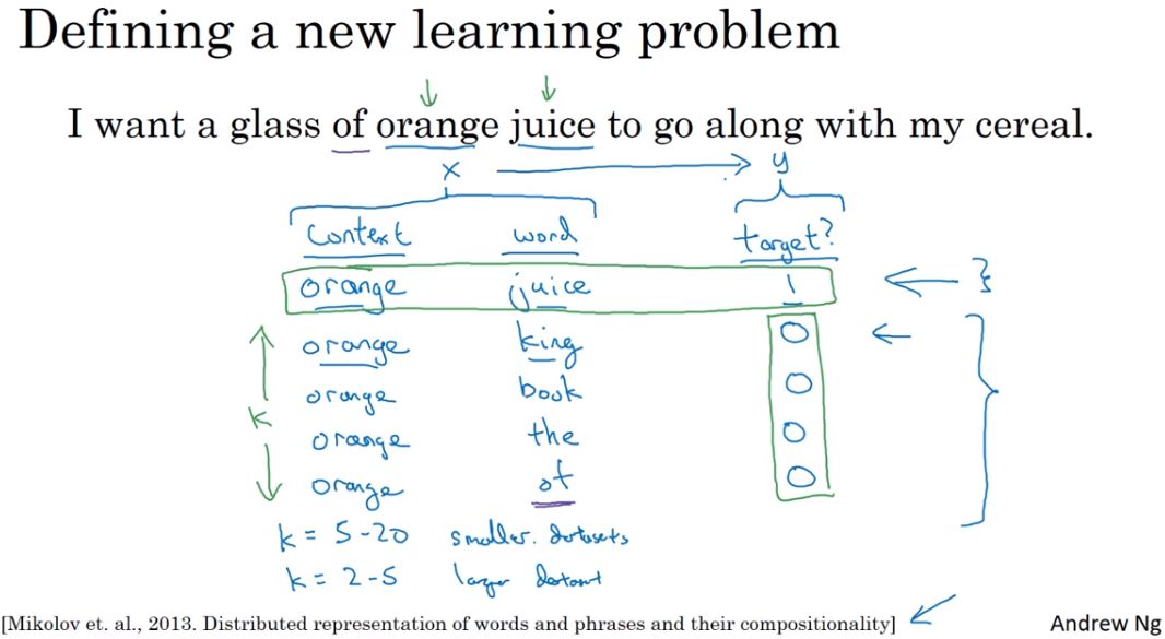
• 负采样：

        1）定义一个新的学习问题：预测两个词是否上下文-目标词对，如果是词对，则标签为1，否则为0。

        2）对同一个上下文，随机选择k个不同的目标词，并且标记标签正负值，生成训练集。小数据集，k=5~20，大数据集，k=2~5。        

        3）模型：将skip-grams模型上下文C是否输出目标词T的概率p(t|c)计算，转化为对C-T为上下文-目标词对时标签为1的概率p(y=1|c,t)的计算，对每一个C，设置了k的词对，因此相对skip-grams计算量减少了。

• Glove模型：怎么实现词嵌入学习的，没咋看懂。。。

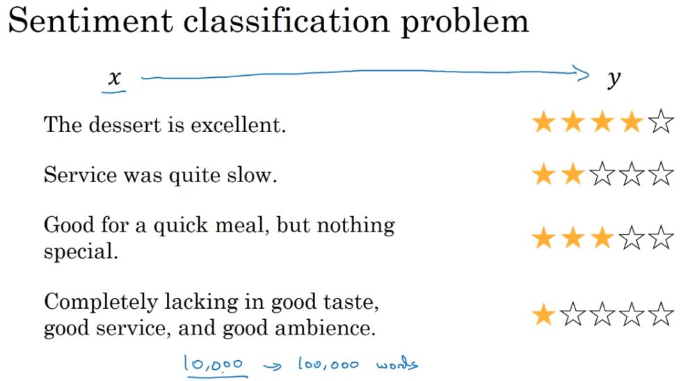
• 情感分类：通过一段文本判断其情感色彩，是喜欢，还是不喜欢。情感分类存在的问题是，只有较小的数据集，缺乏训练集。

        通过词向量平均值做情感分类：这个方法的缺点是没有考虑到词序对情感色彩的影响

        1）对文本的每个词向量化。

        2）对所有词的词向量求和或求平均。

        3）用softmax()分类器输出情感分类概率。

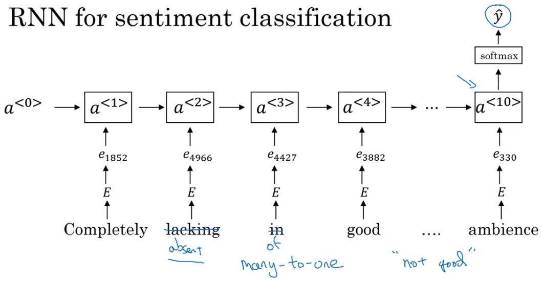
        通过RNN实现情感分类：

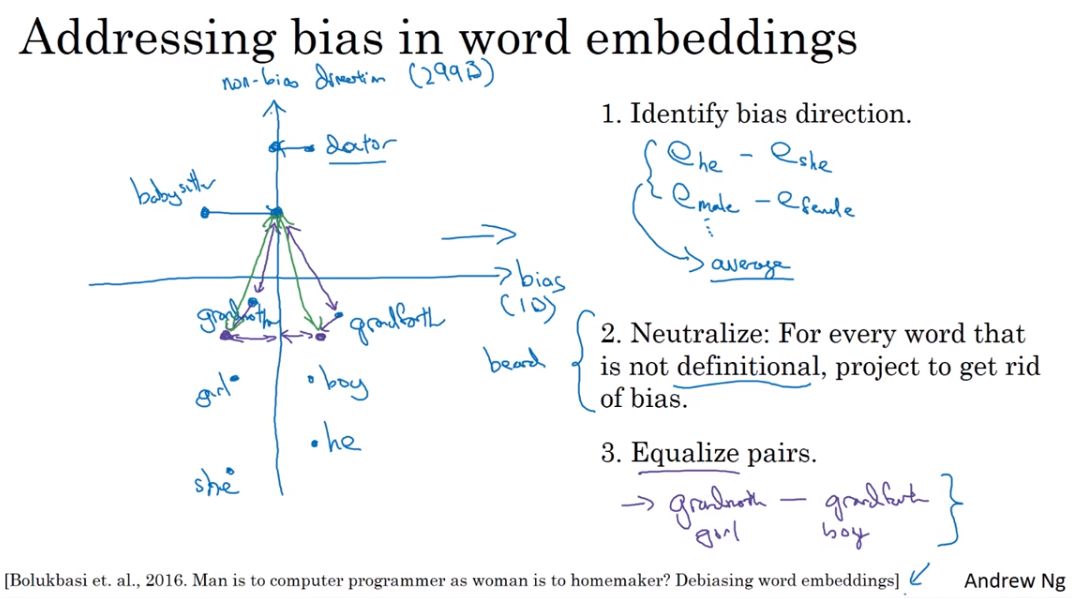
• 词嵌入消除偏见        

        目前存在的社会偏见：

         

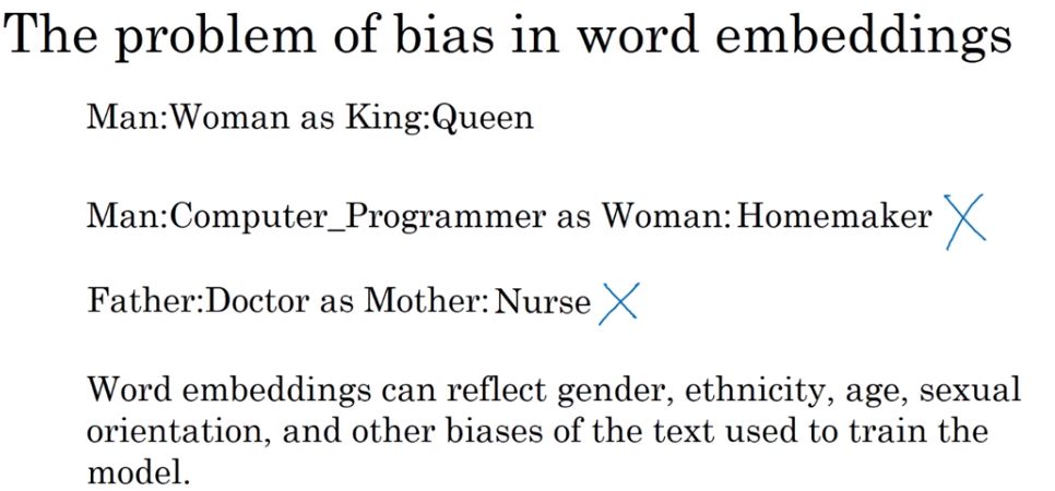
        消除偏见的方法：减去一些词向时中和偏见有关的维度上的值，比如，减去保姆词向量中有关女性的维度

1.2 应用实例：        

实现思路：

• 加载词向量数据（用Glove向量）。
• 计算余弦相似度。

• 求解A对于B，相当于C对于D的问题：

1. 向量化A、B、C。
2. 依次计算词典中的每个一单词word与单词C的差值，并计算A-B和C-word的余弦相似度。
3. 记录最大的相似度，并记录对应单词best_word。
4. 返回best_word。

• 感受词向量的偏见：

1. 计算Vwoman-Vman=g。
2. 分别计算g与常见人句的余弦相似度，结果显示g与女性名字相似度高。
3. 分别计算g与若干个职业的余弦相似度，结果显示g与艺术家、教师余弦相似度高，与科学家、程序员相似度低。

• 消除与性别无关的词汇的偏差：

1. 假设词嵌入向量是50维，其中一维g为性别偏置方向，表示为g，剩下的49维。将e_word沿g方向归零，得到去除偏置方向的向量e_debiased_word。

• 词嵌入向量e，偏置方向g，e在g方向上的投影e_bias=。

• 性别词的均衡算法：

1. 获取两个单词的向量e_w1,e_w2。
2. 计算两个向量的均值mu=（e_w1+e_w2）/2。
3. 计算mu在偏置方向上的投影mu_B。
4. 计算mu在偏置正交轴上的投影mu_orth=mu-mu_B。
5. 计算e_w1,e_w2在偏置轴上的投影，e_w1B,e_w2B。
6. 调整e_w1B,e_w2B的偏置部分（公式的现实意义没看明白？？？？），得corrected_e_w1B,corrected_e_w2B。
7. 修正后的e1=corrected_e_w1B-mu_orth。e2同理。

• V1模型表情生成器：

1. 加载表情训练数据和测试数据。
2. 引入 处理表情的包。
3. 实现基准模型Emojifier_V1。
4. 优化循环，计算每个句子所含单词的平均值，得平均向量avg。前向传播，全连接，softmax()激活。计算损失。计算梯度，更新参数。
5. Emojifier_V1的主要总是是，按句子单词的向量求平均，没有考虑单词顺序对语义的影响。

• V2模型：在keras中使用LSTM

1. 填充句子长度。指定句子最大长度，不中长度的以0填充。以每个句子以相同的长度应用于网络。
2. 将句子单词列表转化为索引列表。
3. 用训练好的词嵌入向量填充嵌入矩阵，embedding_layer。
4. 依次进行LSTM、Dropout和Dense、激活运算。
5. 编译、训练模型。

import numpy as np
import w2v_utils

words, word_to_vec_map = w2v_utils.read_glove_vecs('data/glove.6B.50d.txt')

# python 3.x
print(word_to_vec_map['hello'])

# python 2.x
print word_to_vec_map['hello']

[-0.38497   0.80092   0.064106 -0.28355  -0.026759 -0.34532  -0.64253
 -0.11729  -0.33257   0.55243  -0.087813  0.9035    0.47102   0.56657
  0.6985   -0.35229  -0.86542   0.90573   0.03576  -0.071705 -0.12327
  0.54923   0.47005   0.35572   1.2611   -0.67581  -0.94983   0.68666
  0.3871   -1.3492    0.63512   0.46416  -0.48814   0.83827  -0.9246
 -0.33722   0.53741  -1.0616   -0.081403 -0.67111   0.30923  -0.3923
 -0.55002  -0.68827   0.58049  -0.11626   0.013139 -0.57654   0.048833
  0.67204 ]

def cosine_similarity(u, v):
    """
    u与v的余弦相似度反映了u与v的相似程度
    
    参数：
        u -- 维度为(n,)的词向量
        v -- 维度为(n,)的词向量
        
    返回：
        cosine_similarity -- 由上面公式定义的u和v之间的余弦相似度。
    """
    distance = 0
    
    # 计算u与v的内积
    dot = np.dot(u, v)
    
    #计算u的L2范数
    norm_u = np.sqrt(np.sum(np.power(u, 2)))
    
    #计算v的L2范数
    norm_v = np.sqrt(np.sum(np.power(v, 2)))
    
    # 根据公式1计算余弦相似度
    cosine_similarity = np.divide(dot, norm_u * norm_v)
    
    return cosine_similarity

father = word_to_vec_map["father"]
mother = word_to_vec_map["mother"]
ball = word_to_vec_map["ball"]
crocodile = word_to_vec_map["crocodile"]
france = word_to_vec_map["france"]
italy = word_to_vec_map["italy"]
paris = word_to_vec_map["paris"]
rome = word_to_vec_map["rome"]

print("cosine_similarity(father, mother) = ", cosine_similarity(father, mother))
print("cosine_similarity(ball, crocodile) = ",cosine_similarity(ball, crocodile))
print("cosine_similarity(france - paris, rome - italy) = ",cosine_similarity(france - paris, rome - italy))

cosine_similarity(father, mother) =  0.890903844289
cosine_similarity(ball, crocodile) =  0.274392462614
cosine_similarity(france - paris, rome - italy) =  -0.675147930817

def complete_analogy(word_a, word_b, word_c, word_to_vec_map):
    """
    解决“A与B相比就类似于C与____相比一样”之类的问题
    
    参数：
        word_a -- 一个字符串类型的词
        word_b -- 一个字符串类型的词
        word_c -- 一个字符串类型的词
        word_to_vec_map -- 字典类型，单词到GloVe向量的映射
        
    返回：
        best_word -- 满足(v_b - v_a) 最接近 (v_best_word - v_c) 的词
    """
    
    # 把单词转换为小写
    word_a, word_b, word_c = word_a.lower(), word_b.lower(), word_c.lower()
    
    # 获取对应单词的词向量
    e_a, e_b, e_c = word_to_vec_map[word_a], word_to_vec_map[word_b], word_to_vec_map[word_c]
    
    # 获取全部的单词
    words = word_to_vec_map.keys()
    
    # 将max_cosine_sim初始化为一个比较大的负数
    max_cosine_sim = -100
    best_word = None
    
    # 遍历整个数据集
    for word in words:
        # 要避免匹配到输入的数据
        if word in [word_a, word_b, word_c]:
            continue
        # 计算余弦相似度
        cosine_sim = cosine_similarity((e_b - e_a), (word_to_vec_map[word] - e_c))
        
        if cosine_sim > max_cosine_sim:
            max_cosine_sim = cosine_sim
            best_word = word
            
    return best_word

triads_to_try = [('italy', 'italian', 'spain'), ('india', 'delhi', 'japan'), ('man', 'woman', 'boy'), ('small', 'smaller', 'large')]
for triad in triads_to_try:
    print ('{} -> {} <====> {} -> {}'.format( *triad, complete_analogy(*triad,word_to_vec_map)))

italy -> italian <====> spain -> spanish
india -> delhi <====> japan -> tokyo
man -> woman <====> boy -> girl
small -> smaller <====> large -> larger

triads_to_try = [('small', 'smaller', 'big')]
for triad in triads_to_try:
    print ('{} -> {} <====> {} -> {}'.format( *triad, complete_analogy(*triad,word_to_vec_map)))

g = word_to_vec_map['woman'] - word_to_vec_map['man']
print(g)

[-0.087144    0.2182     -0.40986    -0.03922    -0.1032      0.94165
 -0.06042     0.32988     0.46144    -0.35962     0.31102    -0.86824
  0.96006     0.01073     0.24337     0.08193    -1.02722    -0.21122
  0.695044   -0.00222     0.29106     0.5053     -0.099454    0.40445
  0.30181     0.1355     -0.0606     -0.07131    -0.19245    -0.06115
 -0.3204      0.07165    -0.13337    -0.25068714 -0.14293    -0.224957
 -0.149       0.048882    0.12191    -0.27362    -0.165476   -0.20426
  0.54376    -0.271425   -0.10245    -0.32108     0.2516     -0.33455
 -0.04371     0.01258   ]

name_list = ['john', 'marie', 'sophie', 'ronaldo', 'priya', 'rahul', 'danielle', 'reza', 'katy', 'yasmin']

for w in name_list:
    print (w, cosine_similarity(word_to_vec_map[w], g))

john -0.23163356146
marie 0.315597935396
sophie 0.318687898594
ronaldo -0.312447968503
priya 0.17632041839
rahul -0.169154710392
danielle 0.243932992163
reza -0.079304296722
katy 0.283106865957
yasmin 0.233138577679

word_list = ['lipstick', 'guns', 'science', 'arts', 'literature', 'warrior','doctor', 'tree', 'receptionist', 
             'technology',  'fashion', 'teacher', 'engineer', 'pilot', 'computer', 'singer']
for w in word_list:
    print (w, cosine_similarity(word_to_vec_map[w], g))

lipstick 0.276919162564
guns -0.18884855679
science -0.0608290654093
arts 0.00818931238588
literature 0.0647250443346
warrior -0.209201646411
doctor 0.118952894109
tree -0.0708939917548
receptionist 0.330779417506
technology -0.131937324476
fashion 0.0356389462577
teacher 0.179209234318
engineer -0.0803928049452
pilot 0.00107644989919
computer -0.103303588739
singer 0.185005181365

def neutralize(word, g, word_to_vec_map):
    """
    通过将“word”投影到与偏置轴正交的空间上，消除了“word”的偏差。
    该函数确保“word”在性别的子空间中的值为0
    
    参数：
        word -- 待消除偏差的字符串
        g -- 维度为(50,)，对应于偏置轴（如性别）
        word_to_vec_map -- 字典类型，单词到GloVe向量的映射
        
    返回：
        e_debiased -- 消除了偏差的向量。
    """
    
    # 根据word选择对应的词向量
    e = word_to_vec_map[word]
    
    # 根据公式2计算e_biascomponent
    e_biascomponent = np.divide(np.dot(e, g), np.square(np.linalg.norm(g))) * g
    
    # 根据公式3计算e_debiased
    e_debiased = e - e_biascomponent
    
    return e_debiased

e = "receptionist"
print("去偏差前{0}与g的余弦相似度为：{1}".format(e, cosine_similarity(word_to_vec_map["receptionist"], g)))

e_debiased = neutralize("receptionist", g, word_to_vec_map)
print("去偏差后{0}与g的余弦相似度为：{1}".format(e, cosine_similarity(e_debiased, g)))

去偏差前receptionist与g的余弦相似度为：0.33077941750593737
去偏差后receptionist与g的余弦相似度为：-2.099120994400013e-17

def equalize(pair, bias_axis, word_to_vec_map):
    """
    通过遵循上图中所描述的均衡方法来消除性别偏差。
    
    参数：
        pair -- 要消除性别偏差的词组，比如 ("actress", "actor") 
        bias_axis -- 维度为(50,)，对应于偏置轴（如性别）
        word_to_vec_map -- 字典类型，单词到GloVe向量的映射
    
    返回：
        e_1 -- 第一个词的词向量
        e_2 -- 第二个词的词向量
    """
    # 第1步：获取词向量
    w1, w2 = pair
    e_w1, e_w2 = word_to_vec_map[w1], word_to_vec_map[w2]
    
    # 第2步：计算w1与w2的均值
    mu = (e_w1 + e_w2) / 2.0
    
    # 第3步：计算mu在偏置轴与正交轴上的投影
    mu_B = np.divide(np.dot(mu, bias_axis), np.square(np.linalg.norm(bias_axis))) * bias_axis
    mu_orth = mu - mu_B
    
    # 第4步：使用公式7、8计算e_w1B 与 e_w2B
    e_w1B = np.divide(np.dot(e_w1, bias_axis), np.square(np.linalg.norm(bias_axis))) * bias_axis
    e_w2B = np.divide(np.dot(e_w2, bias_axis), np.square(np.linalg.norm(bias_axis))) * bias_axis
    
    # 第5步：根据公式9、10调整e_w1B 与 e_w2B的偏置部分
    corrected_e_w1B = np.sqrt(np.abs(1-np.square(np.linalg.norm(mu_orth)))) * np.divide(e_w1B-mu_B, np.abs(e_w1 - mu_orth - mu_B))
    corrected_e_w2B = np.sqrt(np.abs(1-np.square(np.linalg.norm(mu_orth)))) * np.divide(e_w2B-mu_B, np.abs(e_w2 - mu_orth - mu_B))
    
    # 第6步： 使e1和e2等于它们修正后的投影之和，从而消除偏差
    e1 = corrected_e_w1B + mu_orth
    e2 = corrected_e_w2B + mu_orth
    
    return e1, e2

print("==========均衡校正前==========")
print("cosine_similarity(word_to_vec_map[\"man\"], gender) = ", cosine_similarity(word_to_vec_map["man"], g))
print("cosine_similarity(word_to_vec_map[\"woman\"], gender) = ", cosine_similarity(word_to_vec_map["woman"], g))
e1, e2 = equalize(("man", "woman"), g, word_to_vec_map)
print("\n==========均衡校正后==========")
print("cosine_similarity(e1, gender) = ", cosine_similarity(e1, g))
print("cosine_similarity(e2, gender) = ", cosine_similarity(e2, g))

==========均衡校正前==========
cosine_similarity(word_to_vec_map["man"], gender) =  -0.117110957653
cosine_similarity(word_to_vec_map["woman"], gender) =  0.356666188463

==========均衡校正后==========
cosine_similarity(e1, gender) =  -0.716572752584
cosine_similarity(e2, gender) =  0.739659647493

import numpy as np
import emo_utils
import emoji
import matplotlib.pyplot as plt

%matplotlib inline

X_train, Y_train = emo_utils.read_csv('data/train_emoji.csv')
X_test, Y_test = emo_utils.read_csv('data/test.csv')

maxLen = len(max(X_train, key=len).split())

index  = 3
print(X_train[index], emo_utils.label_to_emoji(Y_train[index]))

Miss you so much ❤️

Y_oh_train = emo_utils.convert_to_one_hot(Y_train, C=5)
Y_oh_test = emo_utils.convert_to_one_hot(Y_test, C=5)

index = 0 
print("{0}对应的独热编码是{1}".format(Y_train[index], Y_oh_train[index]))

3对应的独热编码是[ 0.  0.  0.  1.  0.]

word_to_index, index_to_word, word_to_vec_map = emo_utils.read_glove_vecs('data/glove.6B.50d.txt')

word = "cucumber"
index = 113317
print("单词{0}对应的索引是：{1}".format(word, word_to_index[word]))
print("索引{0}对应的单词是：{1}".format(index, index_to_word[index]))

单词cucumber对应的索引是：113317
索引113317对应的单词是：cucumber

def sentence_to_avg(sentence, word_to_vec_map):
    """
    将句子转换为单词列表，提取其GloVe向量，然后将其平均。
    
    参数：
        sentence -- 字符串类型，从X中获取的样本。
        word_to_vec_map -- 字典类型，单词映射到50维的向量的字典
        
    返回：
        avg -- 对句子的均值编码，维度为(50,)
    """
    
    # 第一步：分割句子，转换为列表。
    words = sentence.lower().split()
    
    # 初始化均值词向量
    avg = np.zeros(50,)
    
    # 第二步：对词向量取平均。
    for w in words:
        avg += word_to_vec_map[w]
    avg = np.divide(avg, len(words))
    
    return avg

avg = sentence_to_avg("Morrocan couscous is my favorite dish", word_to_vec_map)
print("avg = ", avg)

avg =  [-0.008005    0.56370833 -0.50427333  0.258865    0.55131103  0.03104983
 -0.21013718  0.16893933 -0.09590267  0.141784   -0.15708967  0.18525867
  0.6495785   0.38371117  0.21102167  0.11301667  0.02613967  0.26037767
  0.05820667 -0.01578167 -0.12078833 -0.02471267  0.4128455   0.5152061
  0.38756167 -0.898661   -0.535145    0.33501167  0.68806933 -0.2156265
  1.797155    0.10476933 -0.36775333  0.750785    0.10282583  0.348925
 -0.27262833  0.66768    -0.10706167 -0.283635    0.59580117  0.28747333
 -0.3366635   0.23393817  0.34349183  0.178405    0.1166155  -0.076433
  0.1445417   0.09808667]

def model(X, Y, word_to_vec_map, learning_rate=0.01, num_iterations=400):
    """
    在numpy中训练词向量模型。
    
    参数：
        X -- 输入的字符串类型的数据，维度为(m, 1)。
        Y -- 对应的标签，0-7的数组，维度为(m, 1)。
        word_to_vec_map -- 字典类型的单词到50维词向量的映射。
        learning_rate -- 学习率.
        num_iterations -- 迭代次数。
        
    返回：
        pred -- 预测的向量，维度为(m, 1)。
        W -- 权重参数，维度为(n_y, n_h)。
        b -- 偏置参数，维度为(n_y,)
    """
    np.random.seed(1)
    
    # 定义训练数量
    m = Y.shape[0]
    n_y = 5
    n_h = 50
    
    # 使用Xavier初始化参数
    W = np.random.randn(n_y, n_h) / np.sqrt(n_h)
    b = np.zeros((n_y,))
    
    # 将Y转换成独热编码
    Y_oh = emo_utils.convert_to_one_hot(Y, C=n_y)
    
    # 优化循环
    for t in range(num_iterations):
        for i in range(m):
            # 获取第i个训练样本的均值
            avg = sentence_to_avg(X[i], word_to_vec_map)
            
            # 前向传播
            z = np.dot(W, avg) + b
            a = emo_utils.softmax(z)
            
            # 计算第i个训练的损失
            cost = -np.sum(Y_oh[i]*np.log(a))
            
            # 计算梯度
            dz = a - Y_oh[i]
            dW = np.dot(dz.reshape(n_y,1), avg.reshape(1, n_h))
            db = dz
            
            # 更新参数
            W = W - learning_rate * dW
            b = b - learning_rate * db
        if t % 100 == 0:
            print("第{t}轮，损失为{cost}".format(t=t,cost=cost))
            pred = emo_utils.predict(X, Y, W, b, word_to_vec_map)
            
    return pred, W, b

print(X_train.shape)
print(Y_train.shape)
print(np.eye(5)[Y_train.reshape(-1)].shape)
print(X_train[0])
print(type(X_train))
Y = np.asarray([5,0,0,5, 4, 4, 4, 6, 6, 4, 1, 1, 5, 6, 6, 3, 6, 3, 4, 4])
print(Y.shape)

X = np.asarray(['I am going to the bar tonight', 'I love you', 'miss you my dear',
 'Lets go party and drinks','Congrats on the new job','Congratulations',
 'I am so happy for you', 'Why are you feeling bad', 'What is wrong with you',
 'You totally deserve this prize', 'Let us go play football',
 'Are you down for football this afternoon', 'Work hard play harder',
 'It is suprising how people can be dumb sometimes',
 'I am very disappointed','It is the best day in my life',
 'I think I will end up alone','My life is so boring','Good job',
 'Great so awesome'])

(132,)
(132,)
(132, 5)
never talk to me again
<class 'numpy.ndarray'>
(20,)

pred, W, b = model(X_train, Y_train, word_to_vec_map)

第0轮，损失为1.9520498812810072
Accuracy: 0.348484848485
第100轮，损失为0.07971818726014807
Accuracy: 0.931818181818
第200轮，损失为0.04456369243681402
Accuracy: 0.954545454545
第300轮，损失为0.03432267378786059
Accuracy: 0.969696969697

print("=====训练集====")
pred_train = emo_utils.predict(X_train, Y_train, W, b, word_to_vec_map)
print("=====测试集====")
pred_test = emo_utils.predict(X_test, Y_test, W, b, word_to_vec_map)

=====训练集====
Accuracy: 0.977272727273
=====测试集====
Accuracy: 0.857142857143

X_my_sentences = np.array(["i adore you", "i love you", "funny lol", "lets play with a ball", "food is ready", "you are not happy"])
Y_my_labels = np.array([[0], [0], [2], [1], [4],[3]])

pred = emo_utils.predict(X_my_sentences, Y_my_labels , W, b, word_to_vec_map)
emo_utils.print_predictions(X_my_sentences, pred)

Accuracy: 0.833333333333

i adore you ❤️
i love you ❤️
funny lol ?
lets play with a ball ⚾
food is ready ?
you are not happy ❤️

print(" \t {0} \t {1} \t {2} \t {3} \t {4}".format(emo_utils.label_to_emoji(0), emo_utils.label_to_emoji(1), \
                                                 emo_utils.label_to_emoji(2), emo_utils.label_to_emoji(3), \
                                                 emo_utils.label_to_emoji(4)))
import pandas as pd
print(pd.crosstab(Y_test, pred_test.reshape(56,), rownames=['Actual'], colnames=['Predicted'], margins=True))
emo_utils.plot_confusion_matrix(Y_test, pred_test)

     ❤️      ⚾      ?      ?      ?
Predicted  0.0  1.0  2.0  3.0  4.0  All
Actual                                 
0            6    0    0    1    0    7
1            0    8    0    0    0    8
2            2    0   16    0    0   18
3            1    1    2   12    0   16
4            0    0    1    0    6    7
All          9    9   19   13    6   56

import numpy as np
np.random.seed(0)
import keras
from keras.models import Model
from keras.layers import Dense, Input, Dropout, LSTM, Activation
from keras.layers.embeddings import Embedding
from keras.preprocessing import sequence

np.random.seed(1)
from keras.initializers import glorot_uniform

def sentences_to_indices(X, word_to_index, max_len):
    """
    输入的是X（字符串类型的句子的数组），再转化为对应的句子列表，
    输出的是能够让Embedding()函数接受的列表或矩阵（参见图4）。
    
    参数：
        X -- 句子数组，维度为(m, 1)
        word_to_index -- 字典类型的单词到索引的映射
        max_len -- 最大句子的长度，数据集中所有的句子的长度都不会超过它。
        
    返回：
        X_indices -- 对应于X中的单词索引数组，维度为(m, max_len)
    """
    
    m = X.shape[0]  # 训练集数量
    # 使用0初始化X_indices
    X_indices = np.zeros((m, max_len))
    
    for i in range(m):
        # 将第i个居住转化为小写并按单词分开。
        sentences_words = X[i].lower().split()
        
        # 初始化j为0
        j = 0
        
        # 遍历这个单词列表
        for w in sentences_words:
            # 将X_indices的第(i, j)号元素为对应的单词索引
            X_indices[i, j] = word_to_index[w]
            
            j += 1
            
    return X_indices

X1 = np.array(["funny lol", "lets play baseball", "food is ready for you"])
X1_indices = sentences_to_indices(X1,word_to_index, max_len = 5)
print("X1 =", X1)
print("X1_indices =", X1_indices)

X1 = ['funny lol' 'lets play baseball' 'food is ready for you']
X1_indices = [[ 155345.  225122.       0.       0.       0.]
 [ 220930.  286375.   69714.       0.       0.]
 [ 151204.  192973.  302254.  151349.  394475.]]

def pretrained_embedding_layer(word_to_vec_map, word_to_index):
    """
    创建Keras Embedding()层，加载已经训练好了的50维GloVe向量
    
    参数：
        word_to_vec_map -- 字典类型的单词与词嵌入的映射
        word_to_index -- 字典类型的单词到词汇表（400,001个单词）的索引的映射。
        
    返回：
        embedding_layer() -- 训练好了的Keras的实体层。
    """
    vocab_len = len(word_to_index) + 1
    emb_dim = word_to_vec_map["cucumber"].shape[0]
    
    # 初始化嵌入矩阵
    emb_matrix = np.zeros((vocab_len, emb_dim))
    
    # 将嵌入矩阵的每行的“index”设置为词汇“index”的词向量表示
    for word, index in word_to_index.items():
        emb_matrix[index, :] = word_to_vec_map[word]
    
    # 定义Keras的embbeding层
    embedding_layer = Embedding(vocab_len, emb_dim, trainable=False)
    
    # 构建embedding层。
    embedding_layer.build((None,))
    
    # 将嵌入层的权重设置为嵌入矩阵。
    embedding_layer.set_weights([emb_matrix])
    
    return embedding_layer

embedding_layer = pretrained_embedding_layer(word_to_vec_map, word_to_index)
print("weights[0][1][3] =", embedding_layer.get_weights()[0][1][3])

weights[0][1][3] = -0.3403

def Emojify_V2(input_shape, word_to_vec_map, word_to_index):
    """
    实现Emojify-V2模型的计算图
    
    参数：
        input_shape -- 输入的维度，通常是(max_len,)
        word_to_vec_map -- 字典类型的单词与词嵌入的映射。
        word_to_index -- 字典类型的单词到词汇表（400,001个单词）的索引的映射。
    
    返回：
        model -- Keras模型实体
    """
    # 定义sentence_indices为计算图的输入，维度为(input_shape,)，类型为dtype 'int32' 
    sentence_indices = Input(input_shape, dtype='int32')
    
    # 创建embedding层
    embedding_layer = pretrained_embedding_layer(word_to_vec_map, word_to_index)
    
    # 通过嵌入层传播sentence_indices，你会得到嵌入的结果
    embeddings = embedding_layer(sentence_indices)
    
    # 通过带有128维隐藏状态的LSTM层传播嵌入
    # 需要注意的是，返回的输出应该是一批序列。
    X = LSTM(128, return_sequences=True)(embeddings)
    # 使用dropout，概率为0.5
    X = Dropout(0.5)(X)
    # 通过另一个128维隐藏状态的LSTM层传播X
    # 注意，返回的输出应该是单个隐藏状态，而不是一组序列。
    X = LSTM(128, return_sequences=False)(X)
    # 使用dropout，概率为0.5
    X = Dropout(0.5)(X)
    # 通过softmax激活的Dense层传播X，得到一批5维向量。
    X = Dense(5)(X)
    # 添加softmax激活
    X = Activation('softmax')(X)
    
    # 创建模型实体
    model = Model(inputs=sentence_indices, outputs=X)
    
    return model

model = Emojify_V2((max_Len,), word_to_vec_map, word_to_index)
model.summary()

_________________________________________________________________
Layer (type)                 Output Shape              Param #   
=================================================================
input_1 (InputLayer)         (None, 10)                0         
_________________________________________________________________
embedding_2 (Embedding)      (None, 10, 50)            20000050  
_________________________________________________________________
lstm_1 (LSTM)                (None, 10, 128)           91648     
_________________________________________________________________
dropout_1 (Dropout)          (None, 10, 128)           0         
_________________________________________________________________
lstm_2 (LSTM)                (None, 128)               131584    
_________________________________________________________________
dropout_2 (Dropout)          (None, 128)               0         
_________________________________________________________________
dense_1 (Dense)              (None, 5)                 645       
_________________________________________________________________
activation_1 (Activation)    (None, 5)                 0         
=================================================================
Total params: 20,223,927
Trainable params: 223,877
Non-trainable params: 20,000,050

model.compile(loss='categorical_crossentropy', optimizer='adam', metrics=['accuracy'])

X_train_indices = sentences_to_indices(X_train, word_to_index, maxLen)
Y_train_oh = emo_utils.convert_to_one_hot(Y_train, C = 5)

model.fit(X_train_indices, Y_train_oh, epochs = 50, batch_size = 32, shuffle=True)

Epoch 1/50
132/132 [==============================] - 5s 41ms/step - loss: 1.6106 - acc: 0.1667
Epoch 2/50
132/132 [==============================] - 0s 1ms/step - loss: 1.5380 - acc: 0.3106
Epoch 3/50
132/132 [==============================] - 0s 1ms/step - loss: 1.5063 - acc: 0.3030

...

Epoch 48/50
132/132 [==============================] - 0s 1ms/step - loss: 0.0759 - acc: 0.9697
Epoch 49/50
132/132 [==============================] - 0s 1ms/step - loss: 0.0467 - acc: 0.9924
Epoch 50/50
132/132 [==============================] - 0s 1ms/step - loss: 0.0417 - acc: 0.9848

X_test_indices = sentences_to_indices(X_test, word_to_index, max_len = maxLen)
Y_test_oh = emo_utils.convert_to_one_hot(Y_test, C = 5)
loss, acc = model.evaluate(X_test_indices, Y_test_oh)

print("Test accuracy = ", acc)

56/56 [==============================] - 1s 10ms/step
Test accuracy =  0.928571428571

C = 5
y_test_oh = np.eye(C)[Y_test.reshape(-1)]
X_test_indices = sentences_to_indices(X_test, word_to_index, maxLen)
pred = model.predict(X_test_indices)
for i in range(len(X_test)):
    x = X_test_indices
    num = np.argmax(pred[i])
    if(num != Y_test[i]):
        print('正确表情：'+ emo_utils.label_to_emoji(Y_test[i]) + '   预测结果： '+ X_test[i] + emo_utils.label_to_emoji(num).strip())

正确表情：?   预测结果： work is hard    ?
正确表情：?   预测结果： This girl is messing with me    ❤️
正确表情：❤️   预测结果： I love taking breaks    ?
正确表情：?   预测结果： you brighten my day    ❤️

x_test = np.array(['you are so beautiful'])
X_test_indices = sentences_to_indices(x_test, word_to_index, maxLen)
print(x_test[0] +' '+  emo_utils.label_to_emoji(np.argmax(model.predict(X_test_indices))))

you are so beautiful ❤️