


T-net
transform_nets.py
首先我们来看T-Net模型的代码,它的主要作用是学习出变化矩阵来对输入的点云或特征进行规范化处理。其中包含两个函数,分别是
-
学习点云变换矩阵的:input_transform_net(point_cloud, is_training, bn_decay=None, K=3)
-
学习特征变换矩阵的:feature_transform_net(inputs, is_training, bn_decay=None, K=64)
def input_transform_net(point_cloud, is_training, bn_decay=None, K=3):
    """ Input (XYZ) Transform Net, input is BxNx3 gray image
        Return:
            Transformation matrix of size 3xK """
    batch_size = point_cloud.get_shape()[0].value
    num_point = point_cloud.get_shape()[1].value
pointnet 输入维度?
等待debug
    input_image = tf.expand_dims(point_cloud, -1)
    #转为4D张量,尺寸索引轴从零开始; 如果您指定轴的负数,则从最后向后计数
tf.expand_dims(input, dim, name=None)
e.g.
‘t2’ is a tensor of shape [2, 3, 5]
shape(expand_dims(t2, 0)) --> [1, 2, 3, 5]
shape(expand_dims(t2, 2)) --> [2, 3, 1, 5]
shape(expand_dims(t2, 3)) --> [2, 3, 5, 1]
This operation is useful if you want to add a batch dimension to a single element. For example, if you have a single image of shape [height, width, channels], you can make it a batch of 1 image with expand_dims(image, 0), which will make the shape [1, height, width, channels]
#构建T-Net模型,64--128--1024
    net = tf_util.conv2d(input_image, 64, [1,3],
                         padding='VALID', stride=[1,1],
                         bn=True, is_training=is_training,
                         scope='tconv1', bn_decay=bn_decay)
    net = tf_util.conv2d(net, 128, [1,1],
                         padding='VALID', stride=[1,1],
                         bn=True, is_training=is_training,
                         scope='tconv2', bn_decay=bn_decay)
    net = tf_util.conv2d(net, 1024, [1,1],
                         padding='VALID', stride=[1,1],
                         bn=True, is_training=is_training,
                         scope='tconv3', bn_decay=bn_decay)
其中,tf_util.conv2d是作者自己写的函数,函数声明如下
def conv2d(inputs,
           num_output_channels,
           kernel_size,
           scope,
           stride=[1, 1],
           padding='SAME',
           use_xavier=True,
           stddev=1e-3,
           weight_decay=0.0,
           activation_fn=tf.nn.relu,
           bn=False,
           bn_decay=None,
           is_training=None)
mlp网络的定义如上,其输入为点云数据,每一个点云作为一个batch
- 首先将三通道的点云拓展为4-D的张量,tf.expend_dims()将得到batchn3*1的数据作为网络的输入
- 随后构建网络,利用1*1的卷积来实现全连接。每一层单元依次为64-128-1024-512-256的网络结构
为什么这样?
- 之前的观念是越大的卷积核感受野(receptive field)越大, 看到的信息越多, 提取的特征越好
- 使用多个不同尺寸的卷积核, 提取出不同的特征, 再将这些特征合并起来(在通道维度上). 不同角度的特征的表现一般比单一卷积核要好.
    net = tf_util.max_pool2d(net, [num_point,1],
                             padding='VALID', scope='tmaxpool')
#利用1024维特征生成256维度的特征
    net = tf.reshape(net, [batch_size, -1])
    net = tf_util.fully_connected(net, 512, bn=True, is_training=is_training,
                                  scope='tfc1', bn_decay=bn_decay)
    net = tf_util.fully_connected(net, 256, bn=True, is_training=is_training,
                                  scope='tfc2', bn_decay=bn_decay)

#生成点云旋转矩阵 T=3*3
    with tf.variable_scope('transform_XYZ') as sc:
        assert(K==3)
        weights = tf.get_variable('weights', [256, 3*K],
                                  initializer=tf.constant_initializer(0.0),
                                  dtype=tf.float32)
        biases = tf.get_variable('biases', [3*K],
                                 initializer=tf.constant_initializer(0.0),
                                 dtype=tf.float32)
        biases += tf.constant([1,0,0,0,1,0,0,0,1], dtype=tf.float32)
        transform = tf.matmul(net, weights)
        transform = tf.nn.bias_add(transform, biases)

    transform = tf.reshape(transform, [batch_size, 3, K])
    return transform
通过定义权重[W(256,3K), bais(3K)],将上面的256维特征转变为3*3的旋转矩阵输出。
同样对于特征层的规范化处理,其输入为n64的特征输出为6464的旋转矩阵,网络结构与上面完全相同,只是在输入输出的维度需要变化:
def feature_transform_net(inputs, is_training, bn_decay=None, K=64):
""" Feature Transform Net, input is BxNx1xK
Return:
Transformation matrix of size KxK """
batch_size = inputs.get_shape()[0].value
num_point = inputs.get_shape()[1].value
#构建T-Net模型,64--128--1024
net = tf_util.conv2d(inputs, 64, [1,1],
padding='VALID', stride=[1,1],
bn=True, is_training=is_training,
scope='tconv1', bn_decay=bn_decay)
net = tf_util.conv2d(net, 128, [1,1],
padding='VALID', stride=[1,1],
bn=True, is_training=is_training,
scope='tconv2', bn_decay=bn_decay)
net = tf_util.conv2d(net, 1024, [1,1],
padding='VALID', stride=[1,1],
bn=True, is_training=is_training,
scope='tconv3', bn_decay=bn_decay)
net = tf_util.max_pool2d(net, [num_point,1],
padding='VALID', scope='tmaxpool')
net = tf.reshape(net, [batch_size, -1])
net = tf_util.fully_connected(net, 512, bn=True, is_training=is_training,
scope='tfc1', bn_decay=bn_decay)
net = tf_util.fully_connected(net, 256, bn=True, is_training=is_training,
scope='tfc2', bn_decay=bn_decay)
#生成特征旋转矩阵 T=64*64
with tf.variable_scope('transform_feat') as sc:
weights = tf.get_variable('weights', [256, K*K],
initializer=tf.constant_initializer(0.0),
dtype=tf.float32)
biases = tf.get_variable('biases', [K*K],
initializer=tf.constant_initializer(0.0),
dtype=tf.float32)
biases += tf.constant(np.eye(K).flatten(), dtype=tf.float32)
transform = tf.matmul(net, weights)
transform = tf.nn.bias_add(transform, biases)
transform = tf.reshape(transform, [batch_size, K, K])
return transform
···
mlp网络定义每一层的神经元数量为64--128--512--256。同样在得到256维的特征后利用weight(256\*K\*K), bias(K\*K)来计算出K\*K的**特征旋转矩阵**,其中K为64,为默认输出特征数量。
# MLP处理点云
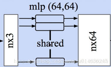
在得到点云的规范化选择矩阵后,将原始输入进行处理。旋转后的点云point_cloud_transformed作为MLP的输入抽取特征。此时输入是旋转后的点云,并通过一个两层的mlp(64--64)得到了64维的特征
# mlp处理特征
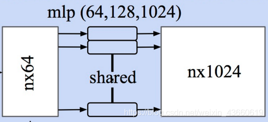
方法同点云
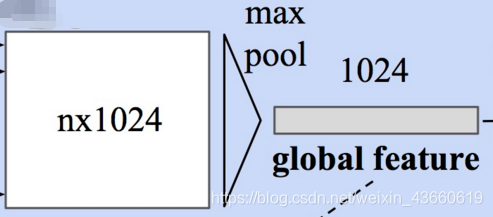
# Max Pooling(对称函数)得到全局特征
此时每个输入点从三维变成了1024维的表示,此时需要对n个点所描述的点云进行融合处理以得到**全局特征**,源码中使用了最大池化层来实现这一功能
```python
# Symmetric function: max pooling
# 最大池化,二维的池化函数对点云中点的数目这个维度进行池化,n-->1
net = tf_util.max_pool2d(net, [num_point,1],
padding='VALID', scope='maxpool')
分类
利用上面的1024维特征,就可以基于这一特征对点云的特性进行学习实现分类任务,PointNet利用了一个三层感知机MPL(512–256–40)来对特征进行学习,最终实现了对于40类的分类.

net = tf.reshape(net, [batch_size, -1])

    # 定义分类的mpl512-256-k, k为分类类别数目
    net = tf_util.fully_connected(net, 512, bn=True, is_training=is_training,
                                  scope='fc1', bn_decay=bn_decay)
    net = tf_util.dropout(net, keep_prob=0.7, is_training=is_training,
                          scope='dp1')
    net = tf_util.fully_connected(net, 256, bn=True, is_training=is_training,
                                  scope='fc2', bn_decay=bn_decay)
    net = tf_util.dropout(net, keep_prob=0.7, is_training=is_training,
                          scope='dp2')
    net = tf_util.fully_connected(net, 40, activation_fn=None, scope='fc3')
分割
对于分割任务,需要加入局域信息来进行学习。所以分类任务的输入包括了1024维的全局信息还包括了n*64的从点云直接学习出的局部信息。PointNet的做法是将全局信息附在每一个局部点描述的后面,形成了1024+64=1088维的向量,而后通过两个感知机来进行分割:

# 定义分割的mpl512-256-128  128-m, m为点所属的类别数目
    net = tf_util.conv2d(concat_feat, 512, [1,1],
                         padding='VALID', stride=[1,1],
                         bn=True, is_training=is_training,
                         scope='conv6', bn_decay=bn_decay)
    net = tf_util.conv2d(net, 256, [1,1],
                         padding='VALID', stride=[1,1],
                         bn=True, is_training=is_training,
                         scope='conv7', bn_decay=bn_decay)
    net = tf_util.conv2d(net, 128, [1,1],
                         padding='VALID', stride=[1,1],
                         bn=True, is_training=is_training,
                         scope='conv8', bn_decay=bn_decay)
    net = tf_util.conv2d(net, 128, [1,1],
                         padding='VALID', stride=[1,1],
                         bn=True, is_training=is_training,
                         scope='conv9', bn_decay=bn_decay)

    net = tf_util.conv2d(net, 50, [1,1],
                         padding='VALID', stride=[1,1], activation_fn=None,
                         scope='conv10')
    net = tf.squeeze(net, [2]) # BxNxC
某些用到的功能
- with … as… 一种初始化语句
- tf作用域
数据集说明
待填充


 4286
4286


 被折叠的 条评论
为什么被折叠?
被折叠的 条评论
为什么被折叠?
 到【灌水乐园】发言


