Pytorch-18种经典的损失函数

最新推荐文章于 2024-06-23 20:57:35 发布

置顶 kaichu2

最新推荐文章于 2024-06-23 20:57:35 发布

阅读量1.1w

点赞数 15

分类专栏： Pytorch 文章标签：深度学习 Pytorch 损失函数

本文链接：https://blog.csdn.net/weixin_43687366/article/details/107927693

版权

Pytorch 专栏收录该内容

30 篇文章 3 订阅

订阅专栏

一、18种损失函数

1、nn.CrossEntropyLoss(交叉熵损失）

（1）什么是熵？：熵是信息论中最基本、最核心的一个概念，它衡量了一个概率分布的随机程度，或者说包含的信息量的大小。

具体公式推导可以参考这篇博主的讲解：一文搞懂交叉损失，讲解浅显易懂！

（2）功能： nn.LogSoftmax ()与nn.NLLLoss ()结合，进行 交叉熵计算

nn.CrossEntropyLoss(weight=None, size_average=None, ignore_index=-100, reduce=None, reduction='mean')

主要参数：

• weight：各类别的loss设置权值

• ignore _index：忽略某个类别

• reduction ：计算模式，可为none/sum /mean

none- 逐个元素计算

sum- 所有元素求和，返回标量

mean- 加权平均，返回标量

其中交叉熵损失数学公式计算如下：

$\text{loss}(x, class) = -\log\left(\frac{\exp(x[class])}{\sum_j \exp(x[j])}\right) | = -x[class] + \log\left(\sum_j \exp(x[j])\right)$ 没有weight的

$\text{loss}(x, class) = weight[class] \left(-x[class] + \log\left(\sum_j \exp(x[j])\right)\right)$ 有weight的

（3）代码实现：对应无参数weight的，不同的计算模式下的结果！

import torch
import torch.nn as nn
import torch.nn.functional as F
import numpy as np

# 输入数据
inputs = torch.tensor([[1,2],[1,3],[1,3]],dtype=torch.float)
# print(inputs)
# 对应输入数据的标签
target = torch.tensor([0,1,1],dtype=torch.long)
# print(target)
print("数据:{0},\n标签:{1}".format(inputs,target))

数据:tensor([[1., 2.],
        [1., 3.],
        [1., 3.]]),
标签:tensor([0, 1, 1])

# CrossEntropy loss: reduction
"""
    reduction有三种计算模式：
    1、none-逐个元素计算
    2、sum-所有元素求和，返回标量
    3、mean-加权平均，返回标量
"""
# flag = 0
flag = 1
if flag:
    # 定义损失函数
    loss_f_none = nn.CrossEntropyLoss(weight=None,reduction='none')
    loss_f_sum = nn.CrossEntropyLoss(weight=None,reduction='sum')
    loss_f_mean = nn.CrossEntropyLoss(weight=None,reduction='mean')
    
    # 前向传播
    loss_none = loss_f_none(inputs,target)
    loss_sum = loss_f_sum(inputs,target)
    loss_mean = loss_f_mean(inputs,target)
    
    # 查看输出结果
    print("Cross Entropy Loss:\n",loss_none)
    print("Cross Entropy Loss:\n",loss_sum)
    print("Cross Entropy Loss:\n",loss_mean)
    
# 手动对上述进行验证
# flag = 0
flag = 1
if flag:
    idx = 0
    # 将tensor转换为数组
    input_1 = inputs.detach().numpy()[idx] # [1,2]数据
    target_1 = target.numpy()[idx] # 0标签
    
    # 第一项
    x_class = input_1[target_1]
    print(x_class)
    
    # 第二项
    sigma_exp_x = np.sum(list(map(np.exp,input_1)))
    log_sigma_exp_x = np.log(sigma_exp_x)
    
    # 输出loss
    loss_1 = -x_class + log_sigma_exp_x
    print("第一个样本loss为：",loss_1)

Cross Entropy Loss:
 tensor([1.3133, 0.1269, 0.1269])
Cross Entropy Loss:
 tensor(1.5671)
Cross Entropy Loss:
 tensor(0.5224)
1.0
第一个样本loss为： 1.3132617

根据系统提供，然后按照手动公式计算，结果是一致的！

# CrossEntropyLoss-------------------有weight参数的------------
# flag = 0
flag = 1
if flag:
    # 定义损失函数
    weights = torch.tensor([1,2],dtype=torch.float)
    loss_f_none_w = nn.CrossEntropyLoss(weight=weights,reduction='none')
    loss_f_sum = nn.CrossEntropyLoss(weight=weights,reduction='sum')
    loss_f_mean = nn.CrossEntropyLoss(weight=weights,reduction='mean')
    
    loss_none_w = loss_f_none_w(inputs,target)
    loss_sum = loss_f_sum(inputs,target)
    loss_mean = loss_f_mean(inputs,target)
    
    print("权重参数：{}".format(weights))
    print("loss_none_w:{}".format(loss_none_w))
    print("loss_sum:{}".format(loss_sum))
    print("loss_mean:{}".format(loss_mean))

# 手动计算验证
# flag = 0
flag = 1
if flag:
    weights = torch.tensor([1,2],dtype=torch.float)
    weights_all = np.sum(list(map(lambda x: weights.numpy()[x],target.numpy())))
    
    mean = 0
    loss_sep = loss_none.detach().numpy()
#     print(loss_sep)
    
    for i in range(target.shape[0]):
        x_class = target.numpy()[i]
        tmp = loss_sep[i]*(weights.numpy()[x_class] / weights_all)
        mean += tmp
        
    print("loss_mean_by_hand:{}".format(mean))

权重参数：tensor([1., 2.])
loss_none_w:tensor([1.3133, 0.2539, 0.2539])
loss_sum:1.8209737539291382
loss_mean:0.36419475078582764
loss_mean_by_hand:0.3641947731375694

2、nn.NLLLoss

NLLLoss(weight=None, size_average=None, ignore_index=-100, reduce=None, reduction='mean')

$\ell(x, y) = L = \{l_1,\dots,l_N\}^\top, \quad l_n = - w_{y_n} x_{n,y_n}, \quad w_{c} = \text{weight}[c] \cdot \mathbb{1}\{c \not= \text{ignore\_index}\}$

#----------------------------NLLLoss--------------------
# flag = 0
flag = 1
if flag:
    weights = torch.tensor([1,1],dtype=torch.float)
    
    loss_f_none_w = nn.NLLLoss(weight=weights,reduction='none')
    loss_none_w = loss_f_none_w(inputs,target)
    
    loss_f_sum = nn.NLLLoss(weight=weights,reduction='sum')
    loss_sum = loss_f_sum(inputs,target)
    
    loss_f_mean = nn.NLLLoss(weight=weights,reduction='mean')
    loss_mean = loss_f_mean(inputs,target)
    print("NLLloss:",loss_none_w.numpy(),loss_sum.numpy(),loss_mean.numpy())

NLL loss: [-1. -3. -3.] -7.0 -2.3333333

3、nn.BCELoss

 BCELoss(weight=None, size_average=None, reduce=None, reduction='mean')

$\ell(x, y) = L = \{l_1,\dots,l_N\}^\top, \quad l_n = - w_n \left[ y_n \cdot \log x_n + (1 - y_n) \cdot \log (1 - x_n) \right]$

N代表batch_size

#-----------------------------BCE Loss------------------------------
# flag = 0
flag = 1
if flag:
    inputs = torch.tensor([[1, 2], [2, 2], [3, 4], [4, 5]], dtype=torch.float)
    target = torch.tensor([[1, 0], [1, 0], [0, 1], [0, 1]], dtype=torch.float)

    target_bce = target

    # itarget
    inputs = torch.sigmoid(inputs)

    weights = torch.tensor([1, 1], dtype=torch.float)

    loss_f_none_w = nn.BCELoss(weight=weights, reduction='none')
    loss_f_sum = nn.BCELoss(weight=weights, reduction='sum')
    loss_f_mean = nn.BCELoss(weight=weights, reduction='mean')

    # forward
    loss_none_w = loss_f_none_w(inputs, target_bce)
    loss_sum = loss_f_sum(inputs, target_bce)
    loss_mean = loss_f_mean(inputs, target_bce)

    # view
    print("\nweights: ", weights)
    print("BCE Loss", loss_none_w, loss_sum, loss_mean)
    

#------------------------手动验证----------------------------------
# flag = 0
flag = 1
if flag:
    idx = 0
    x_i = inputs.detach().numpy()[idx,idx]
    y_i = target.numpy()[idx,idx]
    
    #loss
    # l_i = -[ y_i * np.log(x_i) + (1-y_i) * np.log(1-y_i) ]      # np.log(0) = nan
    l_i = -y_i * np.log(x_i) if y_i else -(1-y-i)*np.log(1-x_i)
    
    print("BCE inputs:",inputs)
    print("第一个loss为：",l_i)

weights:  tensor([1., 1.])
BCE Loss tensor([[0.3133, 2.1269],
        [0.1269, 2.1269],
        [3.0486, 0.0181],
        [4.0181, 0.0067]]) tensor(11.7856) tensor(1.4732)
BCE inputs: tensor([[0.7311, 0.8808],
        [0.8808, 0.8808],
        [0.9526, 0.9820],
        [0.9820, 0.9933]])
第一个loss为： 0.31326166

4、nn.BCEWithLogitsLoss

BCEWithLogitsLoss(weight=None, size_average=None, reduce=None, reduction='mean', pos_weight=None)

$\ell(x, y) = L = \{l_1,\dots,l_N\}^\top, \quad l_n = - w_n \left[ y_n \cdot \log \sigma(x_n) + (1 - y_n) \cdot \log (1 - \sigma(x_n)) \right]$

$\ell(x, y) = \begin{cases} \operatorname{mean}(L), & \text{if reduction} = \text{'mean';}\\ \operatorname{sum}(L), & \text{if reduction} = \text{'sum'.} \end{cases}$

$\ell_c(x, y) = L_c = \{l_{1,c},\dots,l_{N,c}\}^\top, \quad l_{n,c} = - w_{n,c} \left[ p_c y_{n,c} \cdot \log \sigma(x_{n,c}) + (1 - y_{n,c}) \cdot \log (1 - \sigma(x_{n,c})) \right],$

其中c表示多标签分类数，c表示类别，p_c是肯定正确类别c的权重。

其中N代表batch_size，reduction默认是mean

#-------------------------------BCE with Logis Loss-----------------
# flag = 0
flag = 1
if flag:
    inputs = torch.tensor([[1, 2], [2, 2], [3, 4], [4, 5]], dtype=torch.float)
    target = torch.tensor([[1, 0], [1, 0], [0, 1], [0, 1]], dtype=torch.float)

    target_bce = target

    # inputs = torch.sigmoid(inputs)

    weights = torch.tensor([1, 1], dtype=torch.float)

    loss_f_none_w = nn.BCEWithLogitsLoss(weight=weights, reduction='none')
    loss_f_sum = nn.BCEWithLogitsLoss(weight=weights, reduction='sum')
    loss_f_mean = nn.BCEWithLogitsLoss(weight=weights, reduction='mean')

    # forward
    loss_none_w = loss_f_none_w(inputs, target_bce)
    loss_sum = loss_f_sum(inputs, target_bce)
    loss_mean = loss_f_mean(inputs, target_bce)

    # view
    print("\nweights: ", weights)
    print(loss_none_w, loss_sum, loss_mean)

weights:  tensor([1., 1.])
tensor([[0.3133, 2.1269],
        [0.1269, 2.1269],
        [3.0486, 0.0181],
        [4.0181, 0.0067]]) tensor(11.7856) tensor(1.4732)

上面的pos_weight=None取默认值，通过改变pos_weight查看效果如何

# --------------------------------- pos weight

# flag = 0
flag = 1
if flag:
    inputs = torch.tensor([[1, 2], [2, 2], [3, 4], [4, 5]], dtype=torch.float)
    target = torch.tensor([[1, 0], [1, 0], [0, 1], [0, 1]], dtype=torch.float)

    target_bce = target

    # itarget
    # inputs = torch.sigmoid(inputs)

    weights = torch.tensor([1], dtype=torch.float)
    pos_w = torch.tensor([3], dtype=torch.float)        # 3

    loss_f_none_w = nn.BCEWithLogitsLoss(weight=weights, reduction='none', pos_weight=pos_w)
    loss_f_sum = nn.BCEWithLogitsLoss(weight=weights, reduction='sum', pos_weight=pos_w)
    loss_f_mean = nn.BCEWithLogitsLoss(weight=weights, reduction='mean', pos_weight=pos_w)

    # forward
    loss_none_w = loss_f_none_w(inputs, target_bce)
    loss_sum = loss_f_sum(inputs, target_bce)
    loss_mean = loss_f_mean(inputs, target_bce)

    # view
    # 指定第一个位置的权重为3，可以和上面没加权重的结果进行对比
    print("\npos_weights: ", pos_w)
    print(loss_none_w, loss_sum, loss_mean)

pos_weights:  tensor([3.])
tensor([[0.9398, 2.1269],
        [0.3808, 2.1269],
        [3.0486, 0.0544],
        [4.0181, 0.0201]]) tensor(12.7158) tensor(1.5895)

5、nn.L1Loss

功能：计算inputs与target之差的绝对值

L1Loss(size_average=None, reduce=None, reduction='mean')

主要参数：

• reduction ：计算模式，可为none/sum/mean

none- 逐个元素计算

sum- 所有元素求和，返回标量

mean- 加权平均，返回标量

测量输入：x和目标：y中每个元素之间的平均绝对误差（MAE）

$\ell(x, y) = L = \{l_1,\dots,l_N\}^\top, \quad l_n = \left| x_n - y_n \right|$

N代表batch_size，reduction默认是mean

$\ell(x, y) = \begin{cases} \operatorname{mean}(L), & \text{if reduction} = \text{'mean';}\\ \operatorname{sum}(L), & \text{if reduction} = \text{'sum'.} \end{cases}$

求和运算仍然对所有元素进行运算，并除以n。如果设置了 reduction ='sum'，则可以避免除以：n。

#--------------------L1 loss-----------------------------------
inputs = torch.ones((2,2))
target = torch.ones((2,2))*3
loss_f = nn.L1Loss(reduction='none')
loss = loss_f(inputs,target)
# loss = |input-target|
print("input:{}\ntarget:{}\nL1loss:{}".format(inputs,target,loss))

input:tensor([[1., 1.],
        [1., 1.]])
target:tensor([[3., 3.],
        [3., 3.]])
L1loss:tensor([[2., 2.],
        [2., 2.]])

6、nn.MSELoss

功能：计算inputs与target之差的平方；测量输入X中的每个元素与目标Y中的均方误差（L2范数平方）。

主要参数：

• reduction ：计算模式，可为none/sum/mean

none- 逐个元素计算

sum- 所有元素求和，返回标量

mean- 加权平均，返回标量

MSELoss(size_average=None, reduce=None, reduction='mean')

$\ell(x, y) = L = \{l_1,\dots,l_N\}^\top, \quad l_n = \left( x_n - y_n \right)^2$

$\ell(x, y) = \begin{cases} \operatorname{mean}(L), & \text{if reduction} = \text{'mean';}\\ \operatorname{sum}(L), & \text{if reduction} = \text{'sum'.} \end{cases}$

关于reduction种的参数设置和nn.L1loss是一样的！

#----------------------MSE loss----------------------------------
inputs = torch.ones((2,2))
target = torch.ones((2,2))*3
loss_f_mse = nn.MSELoss(reduction='none')
loss_mse = loss_f_mse(inputs,target)
print("MSE Loss:{}".format(loss_mse))

MSE Loss:tensor([[4., 4.],
        [4., 4.]])

7、nn.SmoothL1Loss

是对L1 Loss的一种改进；创建一个使用平方项的标准，如果绝对逐项误差低于1，则使用L1项;否则对异常值的敏感度低于``MSELoss''，并且在某些情况下可以防止梯度爆炸；reduction默认值是均值，和上面几种情况一样！

SmoothL1Loss(size_average=None, reduce=None, reduction='mean')

$\text{loss}(x, y) = \frac{1}{n} \sum_{i} z_{i}$

$z_{i} =\begin{cases} 0.5 (x_i - y_i)^2, & \text{if } |x_i - y_i| < 1 \\ |x_i - y_i| - 0.5, & \text{otherwise } \end{cases}$

#--------------------------------SmoothL1Loss-------------------
# 返回一个一维的tensor（张量），这个张量包含了从start到end（包括端点）的等距的steps个数据点。
inputs = torch.linspace(-3,3,steps=500)
# print(inputs)
target = torch.zeros_like(inputs)
# print(target)
import matplotlib.pyplot as plt
loss_f = nn.SmoothL1Loss(reduction='none')
loss_smooth = loss_f(inputs,target)
loss_l1 = np.abs(inputs.numpy())
plt.plot(inputs.numpy(), loss_smooth.numpy(), label='Smooth L1 Loss')
plt.plot(inputs.numpy(), loss_l1, label='L1 loss')
plt.xlabel('x_i - y_i')
plt.ylabel('loss value')
plt.legend()
plt.grid()
plt.show()

8、PoissonNLLLoss

功能：泊松分布的负对数似然损失函数；

PoissonNLLLoss(log_input=True, full=False, size_average=None, eps=1e-08, reduce=None, reduction='mean')

主要参数：

• log_input ：输入是否为对数形式，决定计算公式

• full ：计算所有loss，默认为False

• eps ：修正项，避免log（input）为nan

$\text{target} \sim \mathrm{Poisson}(\text{input})$

$\text{loss}(\text{input}, \text{target}) = \text{input} - \text{target} * \log(\text{input}) + \log(\text{target!})$

最后一项可以省略，也可以用斯特林公式近似。近似值用于大于1的目标值。对于小于或等于1的目标，将零添加到损耗中。

当 log_input=True 时：

$\text{loss}(\text{input}, \text{target}) = \exp(\text{input}) - \text{target}*\text{input}$

当log_input=False时：

$\text{loss}(\text{input}, \text{target}) = \text{input} - \text{target}*\log(\text{input}+\text{eps})$

#------------------------Poisson NLL loss---------------------------------
inputs = torch.randn((2,2))
target = torch.randn((2,2))
loss_f = nn.PoissonNLLLoss(log_input=True,full=False,reduction='none')
loss = loss_f(inputs,target)
print("input:{}\ntarget:{}\nPoisson NLL loss:{}".format(inputs, target, loss))

#-------------------------手动计算验证-------------------------------------
idx = 0
# 这里的计算参考公式
loss_1 = torch.exp(inputs[idx,idx]) - target[idx,idx]*inputs[idx,idx]
print(inputs[idx,idx])
print("第一个元素loss:", loss_1)

input:tensor([[-2.2698,  1.6573],
        [ 1.9074,  0.3021]])
target:tensor([[ 0.9725, -1.1898],
        [-0.5932, -1.1603]])
Poisson NLL loss:tensor([[2.3108, 7.2171],
        [7.8672, 1.7031]])
tensor(-2.2698)
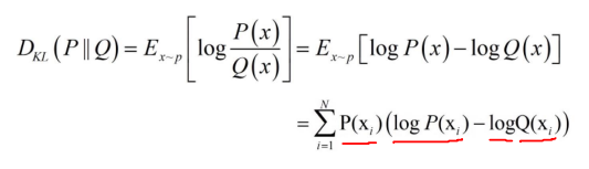
第一个元素loss: tensor(2.3108)

9、nn.KLDivLoss

KLDivLoss(size_average=None, reduce=None, reduction='mean')

KL散度是用于连续分布的有用距离度量，并且在对（离散采样）连续输出分布的空间进行直接回归时通常很有用。

功能：计算KLD（divergence），KL散度，相对 熵

注意事项：需提前将输入计算 log-probabilities， 如通过nn.logsoftmax()

主要参数：

• reduction ：none/sum/mean/batchmean

batchmean- batchsize维度求平均值

none- 逐个元素计算

sum- 所有元素求和，返回标量

mean- 加权平均，返回标量

KL散度的具体描述请看：一文搞懂交叉损失

$l(x,y) = L = \{ l_1,\dots,l_N \}, \quad l_n = y_n \cdot \left( \log y_n - x_n \right)$

$\ell(x, y) = \begin{cases} \operatorname{mean}(L), & \text{if reduction} = \text{'mean';} \\ \operatorname{sum}(L), & \text{if reduction} = \text{'sum'.} \end{cases}$

#-----------------------------------KL Divergence Loss-------------------
inputs = torch.tensor([[0.5, 0.3, 0.2], [0.2, 0.3, 0.5]])
inputs_log = torch.log(inputs)
target = torch.tensor([[0.9, 0.05, 0.05], [0.1, 0.7, 0.2]], dtype=torch.float)

loss_f_none = nn.KLDivLoss(reduction='none')
loss_f_mean = nn.KLDivLoss(reduction='mean')
loss_f_bs_mean = nn.KLDivLoss(reduction='batchmean')

loss_none = loss_f_none(inputs, target)
loss_mean = loss_f_mean(inputs, target)
loss_bs_mean = loss_f_bs_mean(inputs, target)

print("loss_none:\n{}\nloss_mean:\n{}\nloss_bs_mean:\n{}".format(loss_none, loss_mean, loss_bs_mean))

#----------------------------------手动计算验证-------------------------------
idx = 0
# 参考计算公式
loss_1 = target[idx, idx] * (torch.log(target[idx, idx]) - inputs[idx, idx])
print("第一个元素loss:", loss_1)

loss_none:
tensor([[-0.5448, -0.1648, -0.1598],
        [-0.2503, -0.4597, -0.4219]])
loss_mean:
-0.3335360586643219
loss_bs_mean:
-1.000608205795288
第一个元素loss: tensor(-0.5448)

10、nn.MarginRankingLoss

MarginRankingLoss(margin=0.0, size_average=None, reduce=None, reduction='mean')

功能：计算两个向量之间的相似度，用于排序任务

特别说明：该方法计算两组数据之间的差异，返回一个n*n 的 loss 矩阵

主要参数：

• margin ：边界值，x1与x2之间的差异值

• reduction ：计算模式，可为none/sum/mean

$\text{loss}(x, y) = \max(0, -y * (x1 - x2) + \text{margin})$

y = 1时，希望x1比x2大，当x1>x2时，不产生loss

y = -1时，希望x2比x1大，当x2>x1时，不产生loss

#-----------------------------Margin ranking Loss------------------------

x1 = torch.tensor([[1], [2], [3]], dtype=torch.float)
x2 = torch.tensor([[2], [2], [2]], dtype=torch.float)

target = torch.tensor([1, 1, -1], dtype=torch.float)

loss_f_none = nn.MarginRankingLoss(margin=0, reduction='none')

loss = loss_f_none(x1, x2, target)

print(loss)

tensor([[1., 1., 0.],
        [0., 0., 0.],
        [0., 0., 1.]])

11、nn.MultiLabelMarginLoss

MultiLabelMarginLoss(size_average=None, reduce=None, reduction='mean')

optimizes a multi-class multi-classification hinge loss (margin-based loss) between input :math:`x`(a 2D mini-batch `Tensor`) and output :math:`y` ;

$x \in \left\{0, \; \cdots , \; \text{x.size}(0) - 1\right\}$

$y \in \left\{0, \; \cdots , \; \text{y.size}(0) - 1\right\}$

$0 \leq y[j] \leq \text{x.size}(0)-1$

对于所有的 i 和 j 来说；其中x和y的尺寸是相同的；

$i \neq y[j]$

#------------------------Multi label Margin loss-------------------
x = torch.tensor([[0.1, 0.2, 0.4, 0.8]])
y = torch.tensor([[0, 3, -1, -1]], dtype=torch.long)
loss_f = nn.MultiLabelMarginLoss(reduction='none')
loss = loss_f(x, y)
print(loss.squeeze().numpy())

#-------------------------手动验证-------------------------------------
x = x[0]
item_1 = (1-(x[0]-x[1])) + (1-(x[0] - x[2])) # y[0]
item_2 = (1-(x[3] - x[1])) + (1 - (x[3] - x[2]))    # y[3]
loss_h = (item_1 + item_2) / x.shape[0]
print(loss_h.numpy())

0.85
0.85

12、nn.SoftMarginLoss

SoftMarginLoss(size_average=None, reduce=None, reduction='mean')

功能：计算二分类的logistic损失

主要参数：

reduction：计算模式，可为none/sum/mean

$\text{loss}(x, y) = \sum_i \frac{\log(1 + \exp(-y[i]*x[i]))}{\text{x.nelement}()}$

上述x.nelement()统计张量x中的元素个数；

#---------------------------nn.SoftmarginLoss-------------------
inputs = torch.tensor([[0.3, 0.7], [0.5, 0.5]])
target = torch.tensor([[-1, 1], [1, -1]], dtype=torch.float)
loss_f = nn.SoftMarginLoss(reduction='none')
loss = loss_f(inputs, target)
print("softmarginloss:\n{}".format(loss))

#---------------------------compute by hand------------------------
idx = 1
idx1 = 0
inputs_i = inputs[idx,idx1]
# print(inputs_i)
target_i = target[idx,idx1]
loss_hand = np.log(1+np.exp(-target_i*inputs_i))
print(loss_hand)

softmarginloss:
tensor([[0.8544, 0.4032],
        [0.4741, 0.9741]])
tensor(0.4741)

13、nn.MultiLabelSoftMarginLoss

MultiLabelSoftMarginLoss(weight=None, size_average=None, reduce=None, reduction='mean')

功能：SoftMarginLoss多标签版本

主要参数：

weight：各类别的loss设置权值
reduction：计算模式，可为none/sum/mean

$loss(x, y) = - \frac{1}{C} * \sum_i y[i] * \log((1 + \exp(-x[i]))^{-1}) + (1-y[i]) * \log\left(\frac{\exp(-x[i])}{(1 + \exp(-x[i]))}\right)$

其中：

$i \in \left\{0, \; \cdots , \; \text{x.nElement}() - 1\right\}$

$y[i] \in \left\{0, \; 1\right\}$

#------------------------------------Multi Label Softmargin loss---------------
# help(nn.MultiLabelSoftMarginLoss)
inputs = torch.tensor([[0.3, 0.7, 0.8]])
target = torch.tensor([[0, 1, 1]], dtype=torch.float)
loss_f = nn.MultiLabelSoftMarginLoss(reduction='none')
loss = loss_f(inputs, target)
print("MultiLabel SoftMargin: ", loss)
#------------------------------------------------------------------------
i_0 = torch.log(torch.exp(-inputs[0, 0]) / (1 + torch.exp(-inputs[0, 0])))
i_1 = torch.log(1 / (1 + torch.exp(-inputs[0, 1])))
i_2 = torch.log(1 / (1 + torch.exp(-inputs[0, 2])))
loss_h = (i_0 + i_1 + i_2) / -3
print(loss_h)

MultiLabel SoftMargin:  tensor([0.5429])
tensor(0.5429)

14、nn.MultiMarginLoss

MultiLabelMarginLoss(size_average=None, reduce=None, reduction='mean')

功能：计算多分类的折页损失

主要参数：

P：可选1或2
weight：各类别的loss设置权值
margin：边界值
reduction：计算模式，可为none/sum/mean

$\text{loss}(x, y) = \sum_{ij}\frac{\max(0, 1 - (x[y[j]] - x[i]))}{\text{x.size}(0)}$

$x \in \left\{0, \; \cdots , \; \text{x.size}(0) - 1\right\}$ ， $y \in \left\{0, \; \cdots , \; \text{y.size}(0) - 1\right\}$ ， $0 \leq y[j] \leq \text{x.size}(0)-1$ ， $i \neq y[j]$ ，for all i and j

# help(nn.MultiLabelMarginLoss)
x = torch.tensor([[0.1, 0.2, 0.7], [0.2, 0.5, 0.3]])
y = torch.tensor([1, 2], dtype=torch.long)
loss_f = nn.MultiMarginLoss(reduction='none')
loss = loss_f(x, y)
print("Multi Margin Loss: ", loss)

#-----------------------------------------------
x = x[0]
margin = 1
i_0 = margin -(x[1] - x[0])
i_2 = margin - (x[1] - x[2])
loss_h = (i_0 + i_2) / x.shape[0]
print(loss_h)

Multi Margin Loss:  tensor([0.8000, 0.7000])
tensor(0.8000)

15、nn.TripletMarginLoss

TripletMarginLoss(margin=1.0, p=2.0, eps=1e-06, swap=False, size_average=None, reduce=None, reduction='mean')

功能：计算三元组损失，人脸验证中常用；

主要参数：

P范数的阶，默认为2
margin：边界值
reduction：计算模式，可为none/sum/mean

$L(a, p, n) = \max \{d(a_i, p_i) - d(a_i, n_i) + {\rm margin}, 0\}$

$d(x_i, y_i) = \left\lVert {\bf x}_i - {\bf y}_i \right\rVert_p$

其中a，p，n分别表anchor, positive examples and negative examples

# help(nn.TripletMarginLoss)
anchor = torch.tensor([[1.]])
pos = torch.tensor([[2.]])
neg = torch.tensor([[0.5]])
loss_f = nn.TripletMarginLoss(margin=1.0, p=1)
loss = loss_f(anchor, pos, neg)
print("Triplet Margin Loss", loss)

# --------------------------------- compute by hand
margin = 1
a, p, n = anchor[0], pos[0], neg[0]
d_ap = torch.abs(a-p)
d_an = torch.abs(a-n)
loss = d_ap - d_an + margin
print(loss)

Triplet Margin Loss tensor(1.5000)
tensor([1.5000])

16、nn.HingeEmbeddingLoss

 HingeEmbeddingLoss(margin=1.0, size_average=None, reduce=None, reduction='mean')

功能：计算两个输入的相似性，常用于非线性embedding和半监督学习；

特别注意：输入x应为两个输入之差的绝对值

主要参数：

margin：边界值
reduction：计算模式，可为none/sum/mean

The loss function for :math: n-th sample in the mini-batch is:

$l_n = \begin{cases} x_n, & \text{if}\; y_n = 1,\\ \max \{0, \Delta - x_n\}, & \text{if}\; y_n = -1, \end{cases}$

the total loss is: for different reduction

$\ell(x, y) = \begin{cases} \operatorname{mean}(L), & \text{if reduction} = \text{'mean';}\\ \operatorname{sum}(L), & \text{if reduction} = \text{'sum'.} \end{cases}$

$L = \{l_1,\dots,l_N\}^\top$

# help(nn.HingeEmbeddingLoss)
inputs = torch.tensor([[1., 0.8, 0.5]])
target = torch.tensor([[1, 1, -1]])
loss_f = nn.HingeEmbeddingLoss(margin=1, reduction='none')
loss = loss_f(inputs, target)
print("Hinge Embedding Loss", loss)

# --------------------------------- compute by hand
margin = 1.
loss = max(0, margin - inputs.numpy()[0, 2])
print(loss)

Hinge Embedding Loss tensor([[1.0000, 0.8000, 0.5000]])
0.5

17、nn.CosineEmbeddingLoss

 CosineEmbeddingLoss(margin=0.0, size_average=None, reduce=None, reduction='mean')

功能：采用余弦相似度计算两个输入的相似性

主要参数：

margin：可取值 [-1,1]，推荐为 [0,0.5]
reduction：计算模式，可为none/sum/mean

$\text{loss}(x, y) = \begin{cases} 1 - \cos(x_1, x_2), & \text{if } y = 1 \\ \max(0, \cos(x_1, x_2) - \text{margin}), & \text{if } y = -1 \end{cases}$

# help(nn.CosineEmbeddingLoss)
x1 = torch.tensor([[0.3, 0.5, 0.7], [0.3, 0.5, 0.7]])
x2 = torch.tensor([[0.1, 0.3, 0.5], [0.1, 0.3, 0.5]])
target = torch.tensor([[1, -1]], dtype=torch.float)
loss_f = nn.CosineEmbeddingLoss(margin=0., reduction='none')
loss = loss_f(x1, x2, target)
print("Cosine Embedding Loss", loss)

# --------------------------------- compute by hand
margin = 0.
def cosine(a, b):
    numerator = torch.dot(a, b)
    denominator = torch.norm(a, 2) * torch.norm(b, 2)
    return float(numerator/denominator)
l_1 = 1 - (cosine(x1[0], x2[0]))
l_2 = max(0, cosine(x1[0], x2[0]))
print(l_1, l_2)

Cosine Embedding Loss tensor([[0.0167, 0.9833]])
0.016662120819091797 0.9833378791809082

18、nn.CTCLoss

CTCLoss(blank=0, reduction='mean', zero_infinity=False)

功能：计算CTC损失，解决时序类数据的分类

主要参数：

blank：blank label
zero_infinity：无穷大的值或梯度置0
reduction：计算模式，可为none/sum/mean

# help(nn.CTCLoss)
T = 50      # Input sequence length
C = 20      # Number of classes (including blank)
N = 16      # Batch size
S = 30      # Target sequence length of longest target in batch
S_min = 10  # Minimum target length, for demonstration purposes

# Initialize random batch of input vectors, for *size = (T,N,C)
inputs = torch.randn(T, N, C).log_softmax(2).detach().requires_grad_()

# Initialize random batch of targets (0 = blank, 1:C = classes)
target = torch.randint(low=1, high=C, size=(N, S), dtype=torch.long)

input_lengths = torch.full(size=(N,), fill_value=T, dtype=torch.long)
target_lengths = torch.randint(low=S_min, high=S, size=(N,), dtype=torch.long)
ctc_loss = nn.CTCLoss()
loss = ctc_loss(inputs, target, input_lengths, target_lengths)
print("CTC loss: ", loss)

CTC loss:  tensor(5.3379, grad_fn=<MeanBackward0>)

kaichu2

关注

15
点赞
踩
94

收藏

觉得还不错? 一键收藏
打赏
0
评论
复制链接

分享到 QQ

分享到新浪微博

扫一扫

专栏目录

Pytorch-18种经典的损失函数

一、18种损失函数

目录:

1、nn.CrossEntropyLoss(交叉熵损失）

2、nn.NLLLoss

3、nn.BCELoss

4、nn.BCEWithLogitsLoss

5、nn.L1Loss

6、nn.MSELoss

7、nn.SmoothL1Loss

8、PoissonNLLLoss

9、nn.KLDivLoss

10、nn.MarginRankingLoss

11、nn.MultiLabelMarginLoss

12、nn.SoftMarginLoss

13、nn.MultiLabelSoftMarginLoss

14、nn.MultiMarginLoss

15、nn.TripletMarginLoss

16、nn.HingeEmbeddingLoss

17、nn.CosineEmbeddingLoss

18、nn.CTCLoss