【机器学习】鸢尾花Iris数据集进行线性分类

一、实验准备

• 安装python3.6/3.7、Anaconda 和 jupyter、spyder软件。创建一个名为exam1的虚拟环境，在虚拟环境下安装numpy、pandas、sklearn包。按照课件上的代码例子，对鸢尾花Iris数据集进行SVM线性分类练习。
  软件的安装和虚拟环境配置参考了同学的博客【Anaconda】【Jupyter】【Spyder】安装及虚拟环境配置步骤
• 熟悉Jupyter环境下的python编程，在Jupyter下完成一个鸢尾花数据集的线性多分类、可视化显示与测试精度实验。

二、线性分类

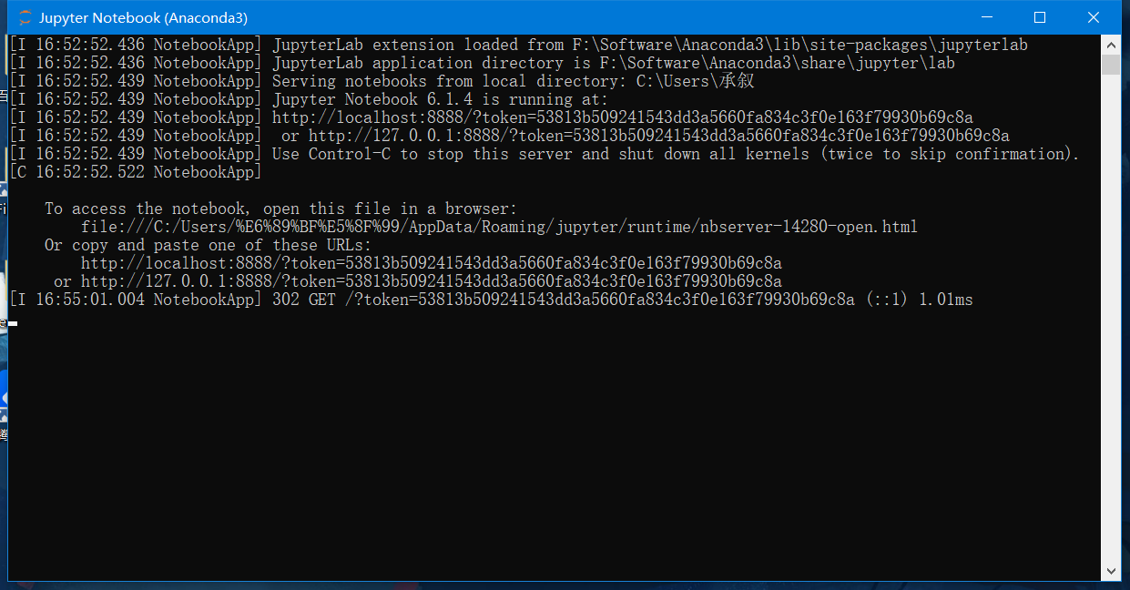
打开Jupyter Notebook

如果未弹出网页，手动将cmd中的网址粘贴到浏览器中即可

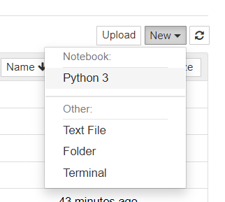
然后在右侧【new】→【python3】

1.原始数据

在代码框内写入以下代码

import numpy as np
import matplotlib.pyplot as plt
from sklearn import datasets
from sklearn.preprocessing import StandardScaler
from sklearn.svm import LinearSVC

iris = datasets.load_iris()
X = iris.data
y = iris.target

X = X [y<2,:2] # 只取y<2的类别，也就是0 1 并且只取前两个特征
y = y[y<2] # 只取y<2的类别

# 分别画出类别 0 和 1 的点
plt.scatter(X[y==0,0],X[y==0,1],color='red')
plt.scatter(X[y==1,0],X[y==1,1],color='blue')
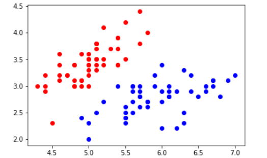
plt.show()

运行结果如下，得出原始数据

2.训练模型

将以下代码添加在上部分代码后面

# 标准化
standardScaler = StandardScaler()
standardScaler.fit(X)

# 计算训练数据的均值和方差
X_standard = standardScaler.transform(X) # 再用 scaler 中的均值和方差来转换 X ，使 X 标准化
svc = LinearSVC(C=1e9) # 线性 SVM 分类器
svc.fit(X_standard,y) # 训练svm

运行结果如下

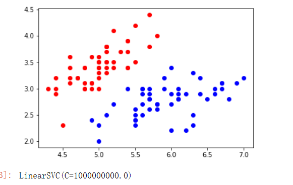
此处C值是控制正则项的重要程度，C越小容错空间越大，求出C=1000000000.0表明模型容错极小。

3.绘制决策边界

同样的，将以下代码添加在上部分代码后面

from matplotlib.colors import ListedColormap # 导入 ListedColormap 包

def plot_decision_boundary(model, axis): 
	x0, x1 = np.meshgrid( np.linspace(axis[0], axis[1], int((axis[1]-axis[0])*100)).reshape(-1,1),
                         np.linspace(axis[2], axis[3], int((axis[3]-axis[2])*100)).reshape(-1,1)
                        )    
	X_new = np.c_[x0.ravel(), x1.ravel()] 
	y_predict = model.predict(X_new) 
	zz = y_predict.reshape(x0.shape) 
	custom_cmap = ListedColormap(['#EF9A9A','#FFF59D','#90CAF9']) 
	plt.contourf(x0, x1, zz, cmap=custom_cmap) #绘制决策边界     
    
plot_decision_boundary(svc,axis=[-3,3,-3,3]) # x,y轴都在-3到3之间 

# 绘制原始数据
plt.scatter(X_standard[y==0,0],X_standard[y==0,1],color='red') 
plt.scatter(X_standard[y==1,0],X_standard[y==1,1],color='blue') 
plt.show()

运行结果如下

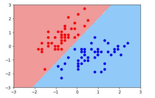
如图，决策边界将两种颜色的点给区分开来了

4.设置参数C

若是上图中，左下角的红点是错误点，决策边界又将是怎么样的？

同样的，将以下代码添加在上部分代码后面，这里一开头就将C值设为0.01，以提高容错

svc2 = LinearSVC(C=0.01)
svc2.fit(X_standard,y)
plot_decision_boundary(svc2,axis=[-3,3,-3,3]) # x,y轴都在-3到3之间
# 绘制原始数据
plt.scatter(X_standard[y==0,0],X_standard[y==0,1],color='red')
plt.scatter(X_standard[y==1,0],X_standard[y==1,1],color='blue')
plt.show()

运行后对比前后两次的结果

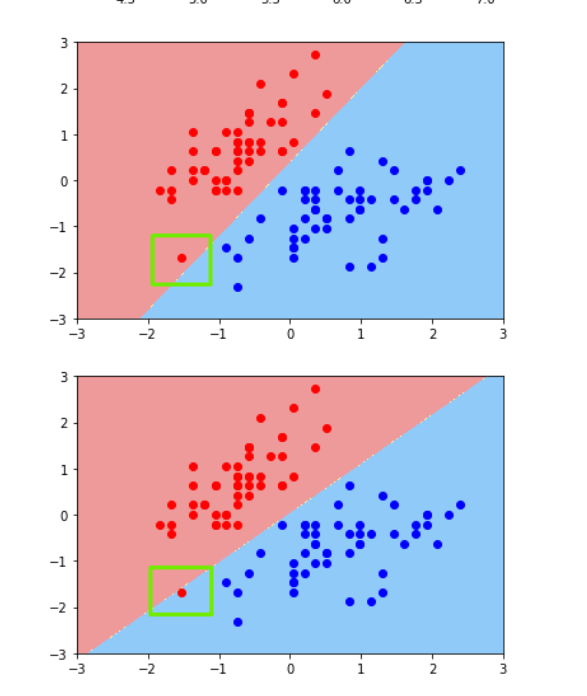
发现当C值设置小了以后，其容错性也增加了，下图的红点也被归为蓝色区域中去了。

三、鸢尾花数据集分类

1.取萼片的长宽作特征分类

1）得到相关数据

#导入相关包
import numpy as np
from sklearn.linear_model import LogisticRegression
import matplotlib.pyplot as plt
import matplotlib as mpl
from sklearn import datasets
from sklearn import preprocessing
import pandas as pd
from sklearn.preprocessing import StandardScaler
from sklearn.pipeline import Pipeline

#获取数据集
df = pd.read_csv('http://archive.ics.uci.edu/ml/machine-learning-databases/iris/iris.data', header=0)
x = df.values[:, :-1]
y = df.values[:, -1]
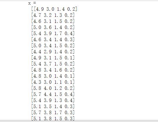
print('x = \n', x)
print('y = \n', y)
le = preprocessing.LabelEncoder()
le.fit(['Iris-setosa', 'Iris-versicolor', 'Iris-virginica'])
print(le.classes_)
y = le.transform(y)
print('Last Version, y = \n', y)

2）处理数据

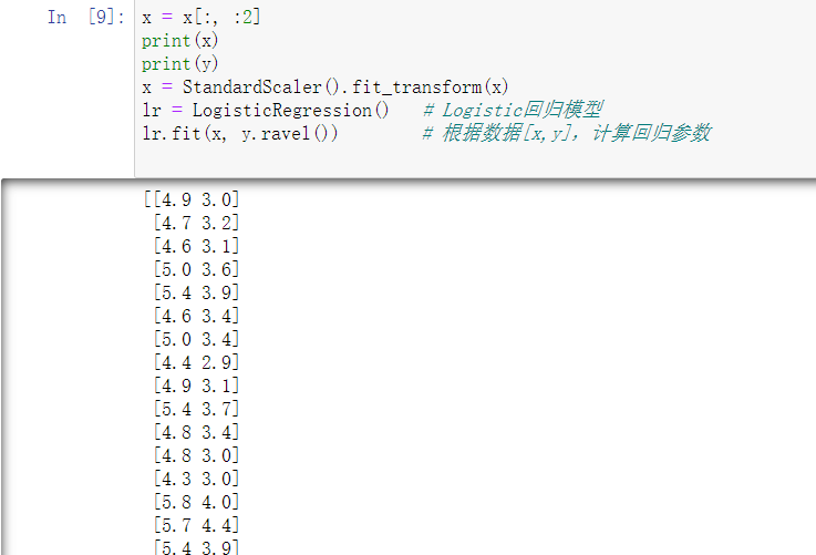
x = x[:, :2] 
print(x)
print(y)
x = StandardScaler().fit_transform(x)
lr = LogisticRegression()   # Logistic回归模型
lr.fit(x, y.ravel())        # 根据数据[x,y]，计算回归参数

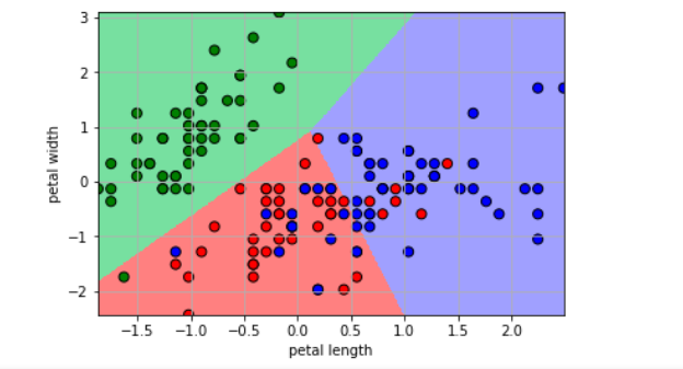
3）绘制图形

N, M = 500, 500     # 横纵各采样多少个值
x1_min, x1_max = X[:, 0].min(), X[:, 0].max()   # 第0列的范围
x2_min, x2_max = X[:, 1].min(), X[:, 1].max()   # 第1列的范围
t1 = np.linspace(x1_min, x1_max, N)
t2 = np.linspace(x2_min, x2_max, M)
x1, x2 = np.meshgrid(t1, t2)                    # 生成网格采样点
x_test = np.stack((x1.flat, x2.flat), axis=1)   # 测试点

cm_light = mpl.colors.ListedColormap(['#77E0A0', '#FF8080', '#A0A0FF'])
cm_dark = mpl.colors.ListedColormap(['g', 'r', 'b'])
y_hat = lr.predict(x_test)       # 预测值
y_hat = y_hat.reshape(x1.shape)                 # 使之与输入的形状相同
plt.pcolormesh(x1, x2, y_hat, cmap=cm_light)     # 预测值的显示
plt.scatter(X[:, 0], X[:, 1], c=Y.ravel(), edgecolors='k', s=50, cmap=cm_dark)    
plt.xlabel('petal length')
plt.ylabel('petal width')
plt.xlim(x1_min, x1_max)
plt.ylim(x2_min, x2_max)
plt.grid()
plt.show()

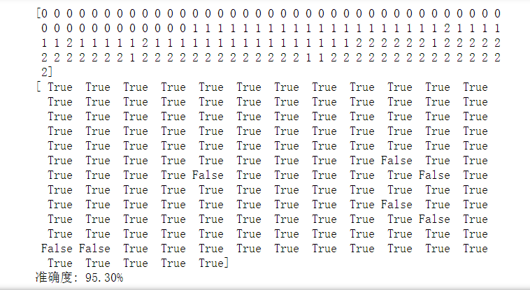
4）预测模型

y_hat = lr.predict(x)
y = y.reshape(-1)
result = y_hat == y
print(y_hat)
print(result)
acc = np.mean(result)
print('准确度: %.2f%%' % (100 * acc))

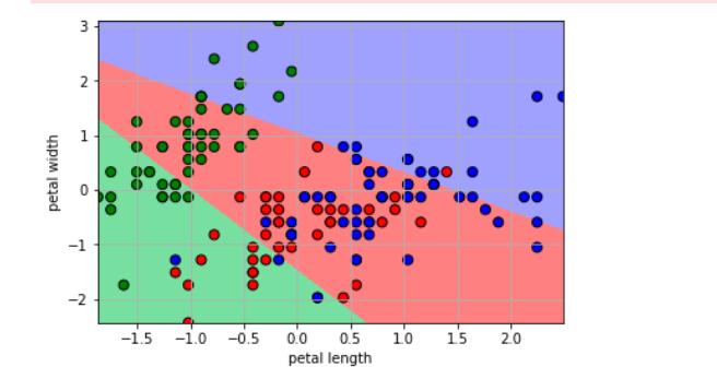
2.取花瓣的长宽作特征分类

其他代码同上，唯独处理数据处代码稍作修改

x = x[:, 2:]    #原本为x = x[:, :2]，后改为x = x[:, 2:]
print(x)
print(y)
x = StandardScaler().fit_transform(x)
lr = LogisticRegression()   # Logistic回归模型
lr.fit(x, y.ravel())        # 根据数据[x,y]，计算回归参数

运行结果如下

四、参考

①【Anaconda】【Jupyter】【Spyder】安装及虚拟环境配置步骤
②从 python 编程角度了解 SVM 对线性与非线性数据分类原理
③对鸢尾花数据集进行线性多分类、可视化显示、测试精度实验