机器学习之线性分类以及Fisher线性判别

机器学习之线性分类以及Fisher线性判别

一、什么是线性分类器和Fisher判别

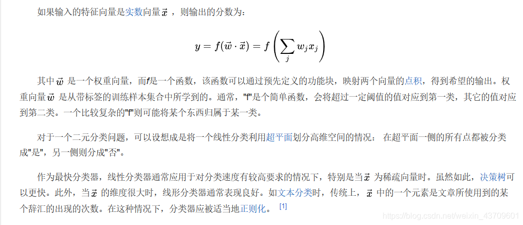
在机器学习领域，分类的目标是指将具有相似特征的对象聚集。而一个线性分类器则透过特征的线性组合来做出分类决定，以达到此种目的。对象的特征通常被描述为特征值，而在向量中则描述为特征向量。

线性分类器定义：

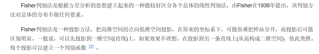
Fisher线性判别：

Fisher判别法是判别分析的方法之一，它是借助于方差分析的思想，利用已知各总体抽取的样品的p维观察值构造一个或多个线性判别函数y=l′x其中l= (l1，l2…lp)′，x= (x1，x2，…，xp)′，使不同总体之间的离差(记为B)尽可能地大，而同一总体内的离差(记为E)尽可能地小来确定判别系数l=(l1，l2…lp)′。数学上证明判别系数l恰好是|B-λE|=0的特征根，记为λ1≥λ2≥…≥λr>0。所对应的特征向量记为l1，l2，…lr，则可写出多个相应的线性判别函数，在有些问题中，仅用一个λ1对应的特征向量l1所构成线性判别函数y1=l′1x不能很好区分各个总体时，可取λ2对应的特征向量l′2建立第二个线性判别函数y2=l′2x，如还不够，依此类推。有了判别函数，再人为规定一个分类原则(有加权法和不加权法等)就可对新样品x判别所属 。

基本介绍：

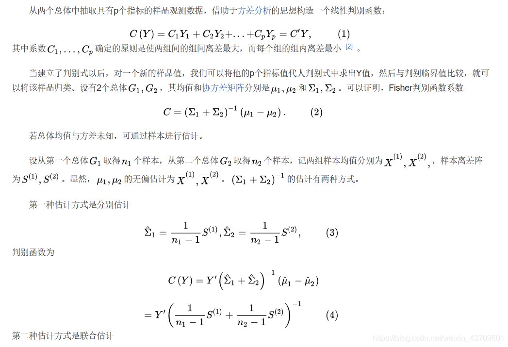
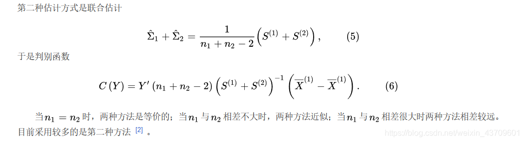
两个总体的Fisher判别函数：

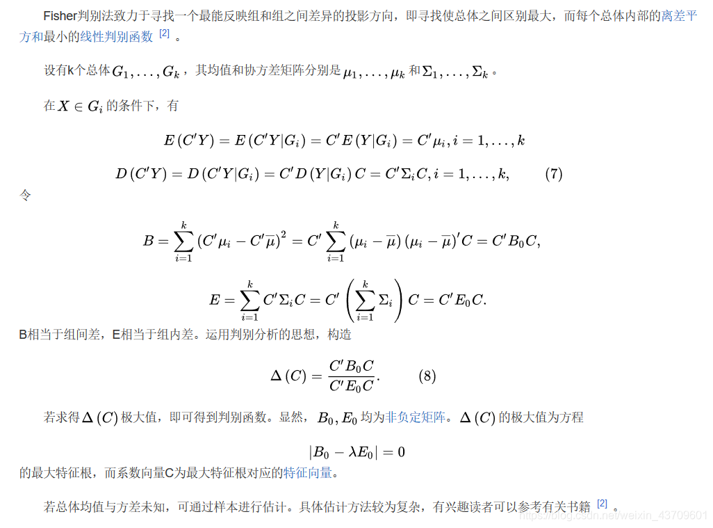
多个总体的Fisher判别函数：

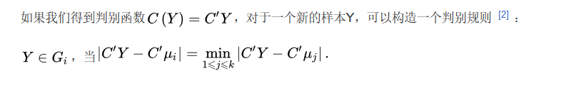
判别规则：

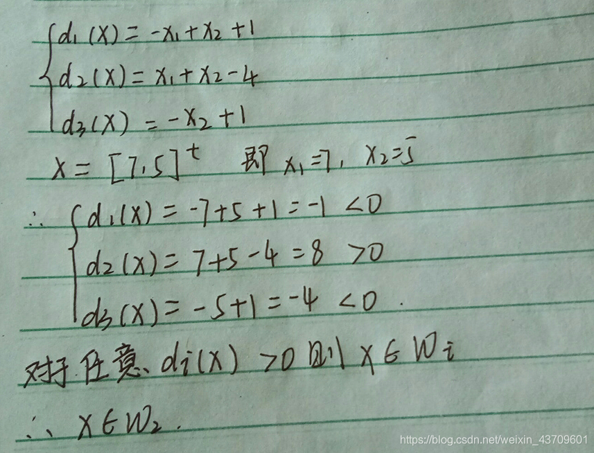
二、判别下一模式属于哪类

三、Fisher判别python代码的推导

Iris数据集的 Fisher线性分类判断及准确率计算:

#导入相关库
import pandas as pd
import numpy as np
import matplotlib.pyplot as plt 
import seaborn as sns

#构建数据集
path=(r'http://archive.ics.uci.edu/ml/machine-learning-databases/iris/iris.data')
df = pd.read_csv(path, header=0)
Iris1=df.values[0:50,0:4]
Iris2=df.values[50:100,0:4]
Iris3=df.values[100:150,0:4]

#构建样本类内离散度矩阵
m1=np.mean(Iris1,axis=0)
m2=np.mean(Iris2,axis=0)
m3=np.mean(Iris3,axis=0)
s1=np.zeros((4,4))
s2=np.zeros((4,4))
s3=np.zeros((4,4))
for i in range(0,30,1):
    a=Iris1[i,:]-m1
    a=np.array([a])
    b=a.T
    s1=s1+np.dot(b,a)    
for i in range(0,30,1):
    c=Iris2[i,:]-m2
    c=np.array([c])
    d=c.T
    s2=s2+np.dot(d,c) 
for i in range(0,30,1):
    a=Iris3[i,:]-m3
    a=np.array([a])
    b=a.T
    s3=s3+np.dot(b,a) 
sw12=s1+s2
sw13=s1+s3
sw23=s2+s3
#投影方向
a=np.array([m1-m2])
sw12=np.array(sw12,dtype='float')
sw13=np.array(sw13,dtype='float')
sw23=np.array(sw23,dtype='float')
#判别函数以及T
a=m1-m2
a=np.array([a])
a=a.T
b=m1-m3
b=np.array([b])
b=b.T
c=m2-m3
c=np.array([c])
c=c.T
w12=(np.dot(np.linalg.inv(sw12),a)).T
w13=(np.dot(np.linalg.inv(sw13),b)).T
w23=(np.dot(np.linalg.inv(sw23),c)).T
T12=-0.5*(np.dot(np.dot((m1+m2),np.linalg.inv(sw12)),a))
T13=-0.5*(np.dot(np.dot((m1+m3),np.linalg.inv(sw13)),b))
T23=-0.5*(np.dot(np.dot((m2+m3),np.linalg.inv(sw23)),c))
#通过判别函数进行判别，求解正确率
kind1=0
kind2=0
kind3=0
newiris1=[]
newiris2=[]
newiris3=[]
for i in range(30,49):
    x=Iris1[i,:]
    x=np.array([x])
    g12=np.dot(w12,x.T)+T12
    g13=np.dot(w13,x.T)+T13
    g23=np.dot(w23,x.T)+T23
    if g12>0 and g13>0:
        newiris1.extend(x)
        kind1=kind1+1
    elif g12<0 and g23>0:
        newiris2.extend(x)
    elif g13<0 and g23<0 :
        newiris3.extend(x)
for i in range(30,49):
    x=Iris2[i,:]
    x=np.array([x])
    g12=np.dot(w12,x.T)+T12
    g13=np.dot(w13,x.T)+T13
    g23=np.dot(w23,x.T)+T23
    if g12>0 and g13>0:
        newiris1.extend(x)
    elif g12<0 and g23>0:
 
        newiris2.extend(x)
        kind2=kind2+1
    elif g13<0 and g23<0 :
        newiris3.extend(x)
for i in range(30,49):
    x=Iris3[i,:]
    x=np.array([x])
    g12=np.dot(w12,x.T)+T12
    g13=np.dot(w13,x.T)+T13
    g23=np.dot(w23,x.T)+T23
    if g12>0 and g13>0:
        newiris1.extend(x)
    elif g12<0 and g23>0:     
        newiris2.extend(x)
    elif g13<0 and g23<0 :
        newiris3.extend(x)
        kind3=kind3+1
correct=(kind1+kind2+kind3)/60
print("样本类内离散度矩阵S1：",s1,'\n')
print("样本类内离散度矩阵S2：",s2,'\n')
print("样本类内离散度矩阵S3：",s3,'\n')
print("总体类内离散度矩阵Sw12：",sw12,'\n')
print("总体类内离散度矩阵Sw13：",sw13,'\n')
print("总体类内离散度矩阵Sw23：",sw23,'\n')
print('判断出来的综合正确率：',correct*100,'%')

样本类内离散度矩阵S1： [[4.084080000000003 2.9814400000000005 0.5409999999999995
  0.4941599999999999]
 [2.9814400000000005 3.6879200000000028 -0.025000000000000428
  0.5628800000000002]
 [0.5409999999999995 -0.025000000000000428 1.0829999999999995 0.19]
 [0.4941599999999999 0.5628800000000002 0.19 0.30832000000000004]] 

样本类内离散度矩阵S2： [[8.316120000000005 2.7365199999999987 5.568960000000003
  1.7302799999999998]
 [2.7365199999999987 3.09192 2.49916 1.3588799999999999]
 [5.568960000000003 2.49916 6.258680000000002 2.2232399999999997]
 [1.7302799999999998 1.3588799999999999 2.2232399999999997
  1.3543200000000004]] 

样本类内离散度矩阵S3： [[14.328471470220745 3.1402832153269435 11.94600583090379
  1.3147563515201988]
 [3.1402832153269435 3.198721366097457 2.239650145772593
  1.2317617659308615]
 [11.94600583090379 2.239650145772593 11.600816326530618
  1.4958892128279884]
 [1.3147563515201988 1.2317617659308615 1.4958892128279884
  1.6810578925447726]] 

总体类内离散度矩阵Sw12： [[12.4002   5.71796  6.10996  2.22444]
 [ 5.71796  6.77984  2.47416  1.92176]
 [ 6.10996  2.47416  7.34168  2.41324]
 [ 2.22444  1.92176  2.41324  1.66264]] 

总体类内离散度矩阵Sw13： [[18.41255147  6.12172322 12.48700583  1.80891635]
 [ 6.12172322  6.88664137  2.21465015  1.79464177]
 [12.48700583  2.21465015 12.68381633  1.68588921]
 [ 1.80891635  1.79464177  1.68588921  1.98937789]] 

总体类内离散度矩阵Sw23： [[22.64459147  5.87680322 17.51496583  3.04503635]
 [ 5.87680322  6.29064137  4.73881015  2.59064177]
 [17.51496583  4.73881015 17.85949633  3.71912921]
 [ 3.04503635  2.59064177  3.71912921  3.03537789]] 

判断出来的综合正确率： 91.66666666666666 %

四、Iris数据集的线性分类以及数据可视化

Iris数据集的线性分类以及数据可视化

#导入相关库
import numpy as np
from sklearn.linear_model import LogisticRegression
import matplotlib.pyplot as plt
import matplotlib as mpl
from sklearn import preprocessing
import pandas as pd
from sklearn.preprocessing import StandardScaler
from sklearn.pipeline import Pipeline

#读取数据
df = pd.read_csv('http://archive.ics.uci.edu/ml/machine-learning-databases/iris/iris.data', header=0)
x = df.values[:, :-1]
y = df.values[:, -1]
le = preprocessing.LabelEncoder()
le.fit(['Iris-setosa', 'Iris-versicolor', 'Iris-virginica'])
y = le.transform(y)

#构建线性模型
x = x[:, :2] 
x = StandardScaler().fit_transform(x)
lr = LogisticRegression()   # Logistic回归模型
lr.fit(x, y.ravel())        # 根据数据[x,y]，计算回归参数

C:\Users\Administrator\Anaconda3\lib\site-packages\sklearn\linear_model\logistic.py:432: FutureWarning: Default solver will be changed to 'lbfgs' in 0.22. Specify a solver to silence this warning.
  FutureWarning)
C:\Users\Administrator\Anaconda3\lib\site-packages\sklearn\linear_model\logistic.py:469: FutureWarning: Default multi_class will be changed to 'auto' in 0.22. Specify the multi_class option to silence this warning.
  "this warning.", FutureWarning)





LogisticRegression(C=1.0, class_weight=None, dual=False, fit_intercept=True,
                   intercept_scaling=1, l1_ratio=None, max_iter=100,
                   multi_class='warn', n_jobs=None, penalty='l2',
                   random_state=None, solver='warn', tol=0.0001, verbose=0,
                   warm_start=False)

#分类及可视化
N, M = 500, 500     # 横纵各采样多少个值
x1_min, x1_max = x[:, 0].min(), x[:, 0].max()   # 第0列的范围
x2_min, x2_max = x[:, 1].min(), x[:, 1].max()   # 第1列的范围
t1 = np.linspace(x1_min, x1_max, N)
t2 = np.linspace(x2_min, x2_max, M)
x1, x2 = np.meshgrid(t1, t2)                    # 生成网格采样点
x_test = np.stack((x1.flat, x2.flat), axis=1)   # 测试点
cm_light = mpl.colors.ListedColormap(['#77E0A0', '#FF8080', '#A0A0FF'])
cm_dark = mpl.colors.ListedColormap(['g', 'r', 'b'])
y_hat = lr.predict(x_test)       # 预测值
y_hat = y_hat.reshape(x1.shape)                 # 使之与输入的形状相同
plt.pcolormesh(x1, x2, y_hat, cmap=cm_light)     # 预测值的显示
plt.scatter(x[:, 0], x[:, 1], c=y.ravel(), edgecolors='k', s=50, cmap=cm_dark)    
plt.xlabel('petal length')
plt.ylabel('petal width')
plt.xlim(x1_min, x1_max)
plt.ylim(x2_min, x2_max)
plt.grid()
plt.savefig('iris.png')
plt.show()
#计算准确率
y_hat = lr.predict(x)
y = y.reshape(-1)
result = y_hat == y
acc = np.mean(result)
print('准确度: %.2f%%' % (100 * acc))

准确度: 79.19%

可以看到，鸢尾花数据集共分为三类，并且不同的数据分布在不同的类别之中，从而达到线性分类器的效果，但是准确率并不高只有79.19%。

数据可视化

from sklearn import datasets
import pandas as pd
import matplotlib.pyplot as plt 
import numpy as np
import seaborn as sns
from mpl_toolkits.mplot3d import Axes3D
iris = datasets.load_iris() 

data1=pd.DataFrame(np.concatenate((iris.data,iris.target.reshape(150,1)),axis=1),
                           columns=np.append(iris.feature_names,'target'))
data1

	sepal length (cm)	sepal width (cm)	petal length (cm)	petal width (cm)	target
0	5.1	3.5	1.4	0.2	0.0
1	4.9	3.0	1.4	0.2	0.0
2	4.7	3.2	1.3	0.2	0.0
3	4.6	3.1	1.5	0.2	0.0
4	5.0	3.6	1.4	0.2	0.0
...	...	...	...	...	...
145	6.7	3.0	5.2	2.3	2.0
146	6.3	2.5	5.0	1.9	2.0
147	6.5	3.0	5.2	2.0	2.0
148	6.2	3.4	5.4	2.3	2.0
149	5.9	3.0	5.1	1.8	2.0

150 rows × 5 columns

data=pd.DataFrame(np.concatenate((iris.data,np.repeat(iris.target_names,50).reshape(150,1)),axis=1),columns=np.append(iris.feature_names,'target'))
data=data.apply(pd.to_numeric,errors='ignore')
data

	sepal length (cm)	sepal width (cm)	petal length (cm)	petal width (cm)	target
0	5.1	3.5	1.4	0.2	setosa
1	4.9	3.0	1.4	0.2	setosa
2	4.7	3.2	1.3	0.2	setosa
3	4.6	3.1	1.5	0.2	setosa
4	5.0	3.6	1.4	0.2	setosa
...	...	...	...	...	...
145	6.7	3.0	5.2	2.3	virginica
146	6.3	2.5	5.0	1.9	virginica
147	6.5	3.0	5.2	2.0	virginica
148	6.2	3.4	5.4	2.3	virginica
149	5.9	3.0	5.1	1.8	virginica

150 rows × 5 columns

sns.pairplot(data.iloc[:,[0,1,4]],hue='target')
sns.pairplot(data.iloc[:,2:5],hue='target')

<seaborn.axisgrid.PairGrid at 0x200fa6d6388>

plt.scatter(data1.iloc[:,0],data1.iloc[:,1],c=data1.target)
plt.xlabel('sepal length (cm)')
plt.ylabel('sepal width (cm)')

Text(0, 0.5, 'sepal width (cm)')