3.机器学习——算法2

1 线性回归

1 定义与公示

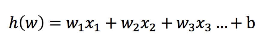
线性回归(Linear regression)是利用回归方程(函数)对一个或多个自变量(特征值)和因变量(目标值)之间关系进行建模的一种分析方式。

• 特点：只有一个自变量的情况称为单变量回归，多于一个自变量情况的叫做多元回归

  

• 线性回归用矩阵表示举例

那么怎么理解呢？我们来看几个例子

• 期末成绩：0.7×考试成绩+0.3×平时成绩
• 房子价格 = 0.02×中心区域的距离 + 0.04×城市一氧化氮浓度 + (-0.12×自住房平均房价) + 0.254×城镇犯罪率

上面两个例子，我们看到特征值与目标值之间建立了一个关系，这个关系可以理解为线性模型

2 线性回归的损失和优化

假设在预测房价的例子中，真实的数据之间存在这样的关系：

真实关系：真实房子价格 = 0.02×中心区域的距离 + 0.04×城市一氧化氮浓度 + (-0.12×自住房平均房价) + 0.254×城镇犯罪率

那么现在呢，我们随意指定一个关系（猜测）

随机指定关系：预测房子价格 = 0.25×中心区域的距离 + 0.14×城市一氧化氮浓度 + 0.42×自住房平均房价 + 0.34×城镇犯

请问这样的话，会发生什么？真实结果与我们预测的结果之间是不是存在一定的误差呢？类似这样样子

既然存在这个误差，那我们就将这个误差给衡量出来

损失函数

总损失定义为：

• yi为第i个训练样本的真实值
• h(xi)为第i个训练样本特征值组合预测函数
• 又称最小二乘法

如何去减少这个损失，使我们预测的更加准确些？既然存在了这个损失，我们一直说机器学习有自动学习的功能，在线性回归这里更是能够体现。这里可以通过一些优化方法去优化（其实是数学当中的求导功能）回归的总损失！！！

优化算法

• 线性回归经常使用的两种优化算法
  • 正规方程
  • 梯度下降法

正规方程：(权重带入公示计算，不用迭代学习)

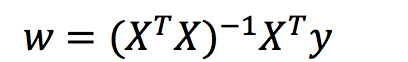
理解：X为特征值矩阵，y为目标值矩阵。直接求到最好的结果

缺点：当特征过多过复杂时，求解速度太慢并且得不到结果

梯度下降

梯度下降法的基本思想可以类比为一个下山的过程。

假设这样一个场景：

一个人被困在山上，需要从山上下来(i.e. 找到山的最低点，也就是山谷)。但此时山上的浓雾很大，导致可视度很低。

因此，下山的路径就无法确定，他必须利用自己周围的信息去找到下山的路径。这个时候，他就可以利用梯度下降算法来帮助自己下山。

具体来说就是，以他当前的所处的位置为基准，寻找这个位置最陡峭的地方，然后朝着山的高度下降的地方走，（同理，如果我们的目标是上山，也就是爬到山顶，那么此时应该是朝着最陡峭的方向往上走）。然后每走一段距离，都反复采用同一个方法，最后就能成功的抵达山谷。

梯度下降的基本过程就和下山的场景很类似。

首先，我们有一个可微分的函数。这个函数就代表着一座山。

我们的目标就是找到这个函数的最小值，也就是山底。

根据之前的场景假设，最快的下山的方式就是找到当前位置最陡峭的方向，然后沿着此方向向下走，对应到函数中，就是找到给定点的梯度 ，然后朝着梯度相反的方向，就能让函数值下降的最快！因为梯度的方向就是函数值变化最快的方向。 所以，我们重复利用这个方法，反复求取梯度，最后就能到达局部的最小值，这就类似于我们下山的过程。而求取梯度就确定了最陡峭的方向，也就是场景中测量方向的手段。

梯度是微积分中一个很重要的概念

在单变量的函数中，梯度其实就是函数的微分，代表着函数在某个给定点的切线的斜率；

在多变量函数中，梯度是一个向量，向量有方向，梯度的方向就指出了函数在给定点的上升最快的方向；

梯度下降和正规方程的对比

梯度下降	正规方程
需要选择学习率	不需要
需要迭代求解	一次运算得出
特征数量较大可以使用	需要计算方程，时间复杂度高O(n3)

算法选择依据

• 小规模数据：
  • 正规方程：LinearRegression(不能解决拟合问题)
  • 岭回归
• 大规模数据：
  • 梯度下降法：SGDRegressor

小结

• 损失函数【知道】
  • 最小二乘法
• 线性回归优化方法【知道】
  • 正规方程
  • 梯度下降法
• 正规方程 – 一蹴而就【知道】
  • 利用矩阵的逆,转置进行一步求解
  • 只是适合样本和特征比较少的情况
• 梯度下降法 — 循序渐进【知道】
  • 梯度的概念
    • 单变量 – 切线
    • 多变量 – 向量
  • 梯度下降法中关注的两个参数
    • α – 就是步长
      • 步长太小 – 下山太慢
      • 步长太大 – 容易跳过极小值点(*****)
    • 为什么梯度要加一个负号
      • 梯度方向是上升最快方向,负号就是下降最快方向
• 梯度下降法和正规方程选择依据【知道】
  • 小规模数据：
    • 正规方程：LinearRegression(不能解决拟合问题)
    • 岭回归
  • 大规模数据：
    • 梯度下降法：SGDRegressor

3 线性回归api介绍

• sklearn.linear_model.LinearRegression(fit_intercept=True)
  • 通过正规方程优化
  • 参数
    • fit_intercept：是否计算偏置
  • 属性
    • LinearRegression.coef_：回归系数
    • LinearRegression.intercept_：偏置
• sklearn.linear_model.SGDRegressor(loss=“squared_loss”, fit_intercept=True, learning_rate =‘invscaling’, eta0=0.01)
  • SGDRegressor类实现了随机梯度下降学习，它支持不同的loss函数和正则化惩罚项来拟合线性回归模型。
  • 参数：
    • loss:损失类型
      • loss=”squared_loss”: 普通最小二乘法
    • fit_intercept：是否计算偏置
    • learning_rate : string, optional
      • 学习率填充
      • ’constant’: eta = eta0
      • ’optimal’: eta = 1.0 / (alpha * (t + t0)) [default]
      • ‘invscaling’: eta = eta0 / pow(t, power_t)
        • power_t=0.25:存在父类当中
      • 对于一个常数值的学习率来说，可以使用learning_rate=’constant’ ，并使用eta0来指定学习率。
  • 属性：
    • SGDRegressor.coef_：回归系数
    • SGDRegressor.intercept_：偏置

sklearn提供给我们两种实现的API， 可以根据选择使用

小结

• 正规方程
  • sklearn.linear_model.LinearRegression()
• 梯度下降法
  • sklearn.linear_model.SGDRegressor(）

4 欠拟合与过拟合

在进行线性回归是可能出现，训练数据训练的很好啊，误差也不大，为什么在测试集上面有问题呢？

• 欠拟合

• 过拟合

• 分析

  • 第一种情况：因为机器学习到的天鹅特征太少了，导致区分标准太粗糙，不能准确识别出天鹅。
  • 第二种情况：机器已经基本能区别天鹅和其他动物了。然后，很不巧已有的天鹅图片全是白天鹅的，于是机器经过学习后，会认为天鹅的羽毛都是白的，以后看到羽毛是黑的天鹅就会认为那不是天鹅。

• 过拟合：一个假设在训练数据上能够获得比其他假设更好的拟合， 但是在测试数据集上却不能很好地拟合数据，此时认为这个假设出现了过拟合的现象。(模型过于复杂)

• 欠拟合：一个假设在训练数据上不能获得更好的拟合，并且在测试数据集上也不能很好地拟合数据，此时认为这个假设出现了欠拟合的现象。(模型过于简单)

原因以及解决办法

• 欠拟合原因以及解决办法
  • 原因：学习到数据的特征过少
  • 解决办法：增加数据的特征数量
• 过拟合原因以及解决办法
  • 原因：原始特征过多，存在一些嘈杂特征， 模型过于复杂是因为模型尝试去兼顾各个测试数据点
  • 解决办法：
    • 正则化

在这里针对回归，我们选择了正则化。但是对于其他机器学习算法如分类算法来说也会出现这样的问题，除了一些算法本身作用之外（决策树、神经网络），我们更多的也是去自己做特征选择，包括之前说的删除、合并一些特征

关于优化方法GD、SGD、SAG

GD

梯度下降(Gradient Descent)，原始的梯度下降法需要计算所有样本的值才能够得出梯度，计算量大，所以后面才有会一系列的改进。

SGD

随机梯度下降(Stochastic gradient descent)是一个优化方法。它在一次迭代时只考虑一个训练样本。

• SGD的优点是：
  • 高效
  • 容易实现
• SGD的缺点是：
  • SGD需要许多超参数：比如正则项参数、迭代数。
  • SGD对于特征标准化是敏感的。

SAG

随机平均梯度法(Stochasitc Average Gradient)，由于收敛的速度太慢，有人提出SAG等基于梯度下降的算法

Scikit-learn：SGDRegressor、岭回归、逻辑回归等当中都会有SAG优化

正则化类别

• L1正则化

  • 作用：可以使得其中一些W的值直接为0，删除这个特征的影响
  • LASSO回归

• L2正则化

  • 作用：可以使得其中一些W的都很小，都接近于0，削弱某个特征的影响
  • 优点：越小的参数说明模型越简单，越简单的模型则越不容易产生过拟合现象
  • Ridge回归

方法选择

总结：

**大数据量：**使用梯度下降发。小数据量：如果少量的重要的特征值使用L1正则化，如果特征比较重要使用L2正则化

5 线性回归的改进

API

• sklearn.linear_model.Ridge(alpha=1.0, fit_intercept=True,solver=“auto”, normalize=False)
  • 具有l2正则化的线性回归
  • alpha:正则化力度，也叫 λ
    • λ取值：0~1 1~10
  • solver:会根据数据自动选择优化方法
    • sag:如果数据集、特征都比较大，选择该随机梯度下降优化
  • normalize:数据是否进行标准化
    • normalize=False:可以在fit之前调用preprocessing.StandardScaler标准化数据
  • Ridge.coef_:回归权重
  • Ridge.intercept_:回归偏置

All last four solvers support both dense and sparse data. However,
only 'sag' supports sparse input when `fit_intercept` is True.

Ridge方法相当于SGDRegressor(penalty=‘l2’, loss=“squared_loss”),只不过SGDRegressor实现了一个普通的随机梯度下降学习，推荐使用Ridge(实现了SAG)

观察正则化程度的变化，对结果的影响？

• 正则化力度越大，权重系数会越小
• 正则化力度越小，权重系数会越大

6 案例

​ 正规方程的优化方法对波士顿房价进行预测

def linear_LinearRegression():
    '''
    正规方程的优化方法对波士顿房价进行预测
    :return:
    '''
    # 1.数据获取
    boston = load_boston()
    # 2.划分数据集
    x_train, x_test, y_train, y_test = train_test_split(boston.data, boston.target, random_state=22)
    # 3.标准化
    transfer = StandardScaler()
    x_train = transfer.fit_transform(x_train)
    x_test = transfer.transform(x_test)
    # 4.预估器
    estimator = LinearRegression()
    estimator.fit(x_train, y_train)
    # 5.得出模型
    print("正规方程-权重系数\n", estimator.coef_)
    print("正规方程-偏置为\n", estimator.intercept_)
    # 6.模型评估
    y_predict = estimator.predict(x_test)
    print("正规方程-预测房价:\n", y_predict)
    error = mean_squared_error(y_test, y_predict)
    print("正规方程-均方误差为:\n", error)

    return None

#输出结果
正规方程-权重系数
 [-0.64817766  1.14673408 -0.05949444  0.74216553 -1.95515269  2.70902585
 -0.07737374 -3.29889391  2.50267196 -1.85679269 -1.75044624  0.87341624
 -3.91336869]
正规方程-偏置为
 22.62137203166228
正规方程-预测房价:
 [28.22944896 31.5122308  21.11612841 32.6663189  20.0023467  19.07315705
 21.09772798 19.61400153 19.61907059 32.87611987 20.97911561 27.52898011
 15.54701758 19.78630176 36.88641203 18.81202132  9.35912225 18.49452615
 30.66499315 24.30184448 19.08220837 34.11391208 29.81386585 17.51775647
 34.91026707 26.54967053 34.71035391 27.4268996  19.09095832 14.92742976
 30.86877936 15.88271775 37.17548808  7.72101675 16.24074861 17.19211608
  7.42140081 20.0098852  40.58481466 28.93190595 25.25404307 17.74970308
 38.76446932  6.87996052 21.80450956 25.29110265 20.427491   20.4698034
 17.25330064 26.12442519  8.48268143 27.50871869 30.58284841 16.56039764
  9.38919181 35.54434377 32.29801978 21.81298945 17.60263689 22.0804256
 23.49262401 24.10617033 20.1346492  38.5268066  24.58319594 19.78072415
 13.93429891  6.75507808 42.03759064 21.9215625  16.91352899 22.58327744
 40.76440704 21.3998946  36.89912238 27.19273661 20.97945544 20.37925063
 25.3536439  22.18729123 31.13342301 20.39451125 23.99224334 31.54729547
 26.74581308 20.90199941 29.08225233 21.98331503 26.29101202 20.17329401
 25.49225305 24.09171045 19.90739221 16.35154974 15.25184758 18.40766132
 24.83797801 16.61703662 20.89470344 26.70854061 20.7591883  17.88403312
 24.28656105 23.37651493 21.64202047 36.81476219 15.86570054 21.42338732
 32.81366203 33.74086414 20.61688336 26.88191023 22.65739323 17.35731771
 21.67699248 21.65034728 27.66728556 25.04691687 23.73976625 14.6649641
 15.17700342  3.81620663 29.18194848 20.68544417 22.32934783 28.01568563
 28.58237108]
正规方程-均方误差为:
 20.627513763095386

梯度下降方程的优化方法对波士顿房价进行预测

def linear_SGDRegressor():
    '''
    梯度下降方程的优化方法对波士顿房价进行预测
    :return:
    '''
    # 1.获取数据
    boston = load_boston()
    # 2.划分数据集
    x_train, x_test, y_train, y_test = train_test_split(boston.data, boston.target, random_state=22)
    # 3.标准化
    transfer = StandardScaler()
    x_train = transfer.fit_transform(x_train)
    x_test = transfer.transform(x_test)
    # 4.预估器
    # loss=“squared_loss”默认最小二乘法损失类型，fit_intercept=True是否计算偏置，learning_rate学习率 具体他将eta0带入公式中，eta0=0.01 penalty="l2" l2岭回归
    estimator = SGDRegressor(learning_rate="constant", eta0=0.01, max_iter=10000)
    estimator.fit(x_train, y_train)
    # 5.得出模型
    print("梯度下降-权重系数\n", estimator.coef_)
    print("梯度下降-偏置为\n", estimator.intercept_)
    # 6.模型评估
    y_predict = estimator.predict(x_test)
    print("梯度下降-预测房价:\n", y_predict)
    error = mean_squared_error(y_test, y_predict)
    print("梯度下降-均方误差为:\n", error)
    return None

梯度下降-权重系数
 [-0.85113405  1.44153333  0.01188209  1.02908265 -1.97340035  3.2750723
 -0.07788144 -3.30555538  2.4019955  -1.72339866 -1.86398835  1.03537908
 -3.95895425]
梯度下降-偏置为
 [22.81118905]
梯度下降-预测房价:
 [28.8444633  32.14336204 20.93417969 34.45733359 20.10022499 18.84742704
 20.75201297 19.2094298  19.45837032 33.84231996 20.7479124  27.93627753
 15.22447376 20.09369327 38.6399797  17.72479263  8.67897905 18.21489096
 31.54076018 24.36760601 19.04342625 35.46568816 31.34954069 16.86806663
 36.13969044 26.36093789 36.32942801 28.03304196 18.95171077 14.65289753
 31.93115276 15.58571756 39.61802719  4.81288268 16.02124728 16.83600487
  5.70197667 19.85069818 43.3429082  29.53972564 25.40924911 17.44809186
 42.02178552  5.33697946 21.51721917 25.19400611 20.94563862 20.79403492
 17.7481464  26.54641061  8.15078943 27.78980151 32.17337343 16.05184428
  8.23499375 36.81703184 33.60620568 21.90840752 17.3682518  22.23896695
 23.58568325 23.85376084 19.84040793 40.21401249 24.85502637 19.8192781
 13.47216583  4.79964636 45.4267482  21.74431648 15.70698614 22.53677343
 43.00914715 21.35188947 38.4307335  27.20520056 21.70143039 19.95073375
 25.35622234 22.69839952 31.90397646 20.05996079 25.10096329 33.57004171
 27.33728601 20.76771844 29.34967417 21.92512619 26.75068357 20.02240595
 26.30265512 25.24957248 20.09242748 14.50412081 14.82981097 17.9292777
 24.71776362 15.77607837 21.03868649 27.16364523 20.99170348 17.78574762
 24.35580141 23.28602864 21.45983017 39.07139059 15.38457368 21.31655215
 34.02719902 35.30697204 20.26881559 27.37944057 24.00941337 16.93960438
 21.35570787 22.53355941 29.06030844 26.33172411 23.61595568 13.81052302
 13.52626044  1.54696874 29.38455095 20.77677013 22.14585272 28.3604697
 28.81084868]
梯度下降-均方误差为:
 21.341362023687118

岭回归方程的优化方法对波士顿房价进行预测

def linear_ridge():
    '''
    岭回归方程的优化方法对波士顿房价进行预测
    :return:
    '''
    # 1.获取数据
    boston = load_boston()
    # 2.划分数据集
    x_train, x_test, y_train, y_test = train_test_split(boston.data, boston.target, random_state=22)
    # 3.标准化
    transfer = StandardScaler()
    x_train = transfer.fit_transform(x_train)
    x_test = transfer.transform(x_test)
    # 4.预估器
    # loss=“squared_loss”默认最小二乘法损失类型，fit_intercept=True是否计算偏置，learning_rate学习率 具体他将eta0带入公式中，eta0=0.01 penalty="l2" l2岭回归
     estimator = Ridge(alpha=0.05, max_iter=10000)
     estimator.fit(x_train, y_train)

    # 5.得出模型
    print("岭回归-权重系数\n", estimator.coef_)
    print("岭回归-偏置为\n", estimator.intercept_)
    # 6.模型评估
    y_predict = estimator.predict(x_test)
    print("岭回归-预测房价:\n", y_predict)
    #均方误差
    error = mean_squared_error(y_test, y_predict)#每个样本的 （预测值-平均值）平方 再求平均值
    print("岭回归-均方误差为:\n", error)
    return None

岭回归-权重系数
 [-0.64754224  1.14540921 -0.06125928  0.74238156 -1.95329931  2.70955709
 -0.0778145  -3.29686197  2.49801485 -1.8522161  -1.75005797  0.87334654
 -3.91257314]
岭回归-偏置为
 22.62137203166228
岭回归-预测房价:
 [28.22904393 31.5115752  21.11774475 32.66548885 20.00425957 19.07308114
 21.09881912 19.61422697 19.62046442 32.87412797 20.98077177 27.52644906
 15.54761776 19.78722073 36.88531063 18.81112362  9.36238388 18.49585623
 30.66532656 24.30208613 19.0819906  34.1125906  29.81180242 17.51704539
 34.90860535 26.54844401 34.70755275 27.42701782 19.09072722 14.93365851
 30.86781583 15.87673339 37.17620257  7.72607205 16.24266927 17.19020002
  7.4236797  20.00858331 40.58333654 28.9334075  25.25412653 17.75021031
 38.76540896  6.87989725 21.80263856 25.28944505 20.42984728 20.47075023
 17.25307558 26.12410209  8.48931502 27.50675123 30.58261907 16.56093749
  9.39091154 35.54247301 32.29320504 21.81914993 17.60351155 22.08058096
 23.49309529 24.10495987 20.13637981 38.5238939  24.58892271 19.77985231
 13.93588195  6.75534826 42.03779553 21.92166523 16.91183233 22.58441937
 40.76353387 21.40229717 36.89762624 27.19166196 20.98539918 20.38071587
 25.35392252 22.19609792 31.13439562 20.39440664 23.99260724 31.54705647
 26.74749778 20.90157052 29.08108823 21.98456191 26.29253831 20.16675967
 25.49084659 24.09115255 19.90743674 16.35772476 15.25325282 18.40698767
 24.83644322 16.61733201 20.89311786 26.70833021 20.75847937 17.88460842
 24.28517854 23.37553964 21.63554045 36.81207878 15.86759289 21.42890964
 32.81229799 33.73813707 20.6168807  26.87680865 22.66096896 17.35977704
 21.67666736 21.65243443 27.66723586 25.04903676 23.73903438 14.66380087
 15.17877986  3.81633    29.18119976 20.68511078 22.32957975 28.01553368
 28.57978155]
岭回归-均方误差为:
 20.628918415070476

2 分类算法-逻辑回归与二分类

1 逻辑回归的原理

输入

逻辑回归的输入就是一个线性回归的结果。

激活函数

• sigmoid函数

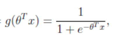
• 分析
  • 回归的结果输入到sigmoid函数当中
  • 输出结果：[0, 1]区间中的一个概率值，默认为0.5为阈值

逻辑回归最终的分类是通过属于某个类别的概率值来判断是否属于某个类别，并且这个类别默认标记为1(正例),另外的一个类别会标记为0(反例)。（方便损失计算）

输出结果解释(重要)：假设有两个类别A，B，并且假设我们的概率值为属于A(1)这个类别的概率值。现在有一个样本的输入到逻辑回归输出结果0.6，那么这个概率值超过0.5，意味着我们训练或者预测的结果就是A(1)类别。那么反之，如果得出结果为0.3那么，训练或者预测结果就为B(0)类别。

所以接下来我们回忆之前的线性回归预测结果我们用均方误差衡量，那如果对于逻辑回归，我们预测的结果不对该怎么去衡量这个损失呢？我们来看这样一张图

2 损失以及优化

损失

逻辑回归的损失，称之为对数似然损失，公式如下：

• 分开类别：

怎么理解单个的式子呢？这个要根据log的函数图像来理解

• 综合完整损失函数

看到这个式子，其实跟我们讲的信息熵类似。

接下来我们呢就带入上面那个例子来计算一遍，就能理解意义了。

我们已经知道，log§, P值越大，结果越小，所以我们可以对着这个损失的式子去分析

优化

同样使用梯度下降优化算法，去减少损失函数的值。这样去更新逻辑回归前面对应算法的权重参数，提升原本属于1类别的概率，降低原本是0类别的概率。

3 逻辑回归API

• sklearn.linear_model.LogisticRegression(solver=‘liblinear’, penalty=‘l2’, C = 1.0)
  • solver:优化求解方式（默认开源的liblinear库实现，内部使用了坐标轴下降法来迭代优化损失函数）
    • sag：根据数据集自动选择，随机平均梯度下降
  • penalty：正则化的种类
  • C：正则化力度

默认将类别数量少的当做正例

LogisticRegression方法相当于 SGDClassifier(loss=“log”, penalty=" "),SGDClassifier实现了一个普通的随机梯度下降学习，也支持平均随机梯度下降法（ASGD），可以通过设置average=True。而使用LogisticRegression(实现了SAG)

4 案例

import pandas as pd
import numpy as np

# 1.读取数据
path = "../resource/cancer/breast-cancer-wisconsin.data"
column_name = ["Sample code number", "Clump Thickness", "Uniformity of Cell Size", "Uniformity of Cell Shape",
               "Marginal Adhesion", "Single Epithelial Cell Size",
               "Bare Nuclei", "Bland Chromatin", "Normal Nucleoli", "Mitoses", "Class"]
data = pd.read_csv(path, names=column_name)

data.head()

	Sample code number	Clump Thickness	Uniformity of Cell Size	Uniformity of Cell Shape	Marginal Adhesion	Single Epithelial Cell Size	Bare Nuclei	Bland Chromatin	Normal Nucleoli	Mitoses	Class
0	1000025	5	1	1	1	2	1	3	1	1	2
1	1002945	5	4	4	5	7	10	3	2	1	2
2	1015425	3	1	1	1	2	2	3	1	1	2
3	1016277	6	8	8	1	3	4	3	7	1	2
4	1017023	4	1	1	3	2	1	3	1	1	2

# 2.数据处理
# 1)替换-》np.nan
data = data.replace(to_replace="?", value=np.nan)
# 2)删除缺失样本
data.dropna(inplace=True)

data.isnull().any()  # 说明不存在缺失值了

Sample code number             False
Clump Thickness                False
Uniformity of Cell Size        False
Uniformity of Cell Shape       False
Marginal Adhesion              False
Single Epithelial Cell Size    False
Bare Nuclei                    False
Bland Chromatin                False
Normal Nucleoli                False
Mitoses                        False
Class                          False
dtype: bool

# 3)筛选特征值和目标值
x = data.iloc[:, 1:-1]
y = data["Class"]

x.head()

	Clump Thickness	Uniformity of Cell Size	Uniformity of Cell Shape	Marginal Adhesion	Single Epithelial Cell Size	Bare Nuclei	Bland Chromatin	Normal Nucleoli	Mitoses
0	5	1	1	1	2	1	3	1	1
1	5	4	4	5	7	10	3	2	1
2	3	1	1	1	2	2	3	1	1
3	6	8	8	1	3	4	3	7	1
4	4	1	1	3	2	1	3	1	1

y.head()

0    2
1    2
2    2
3    2
4    2
Name: Class, dtype: int64

# 4).划分数据集
from sklearn.model_selection import train_test_split
x_train, x_test, y_train, y_test = train_test_split(x, y)

# 3.特征工程 标准化
from sklearn.preprocessing import StandardScaler

transfer = StandardScaler()
x_train = transfer.fit_transform(x_train)
x_test = transfer.transform(x_test)

x_train

array([[-1.19156094, -0.67318491, -0.71103794, ..., -0.98062286,
        -0.59894019, -0.35520315],
       [ 1.29710713, -0.00843916,  0.6473629 , ..., -0.98062286,
         1.07861658,  0.197575  ],
       [-1.19156094, -0.67318491, -0.71103794, ..., -0.98062286,
        -0.59894019, -0.35520315],
       ...,
       [-1.19156094,  0.32393372, -0.03183752, ...,  0.68189007,
         1.07861658, -0.35520315],
       [-1.19156094, -0.67318491, -0.71103794, ..., -0.1493664 ,
        -0.59894019, -0.35520315],
       [ 2.00815515,  2.31817098,  2.34536395, ...,  0.26626184,
         2.420662  ,  4.6198002 ]])

x_test

array([[ 0.2305351 , -0.67318491, -0.71103794, ..., -0.98062286,
        -0.59894019, -0.35520315],
       [-1.19156094, -0.34081203, -0.71103794, ..., -0.56499463,
        -0.59894019, -0.35520315],
       [-1.19156094, -0.67318491, -0.37143773, ..., -0.56499463,
        -0.59894019, -0.35520315],
       ...,
       [-0.48051292, -0.00843916,  0.6473629 , ...,  1.51314653,
        -0.59894019, -0.35520315],
       [-0.48051292, -0.67318491, -0.71103794, ..., -0.56499463,
        -0.59894019, -0.35520315],
       [ 2.00815515, -0.00843916, -0.03183752, ...,  1.51314653,
         0.07208252,  0.75035315]])

# 4 机器学习算法训练 - 模型
from sklearn.linear_model import LogisticRegression

# 1) 逻辑回归预估器
estimator = LogisticRegression()
estimator.fit(x_train, y_train)

LogisticRegression()

# 2)逻辑回归的模型参数 ：回归系数
estimator.coef_

array([[1.36138109, 0.99126667, 0.75422055, 0.71020172, 0.21070533,
        1.00476737, 1.02649748, 0.20188277, 0.426596  ]])

estimator.intercept_

array([-1.33967666])

# 5.模型评估
# 1）直接对比准确率
y_predict = estimator.predict(x_test)
print("y_predict:\n", y_predict)
print("对比真实值和预测值\n", y_predict == y_test)

score = estimator.score(x_test, y_test)
print("准确率为:\n", score)

y_predict:
 [2 2 2 2 2 4 2 4 4 2 4 4 2 2 2 2 2 2 2 2 4 2 2 2 4 2 2 4 4 2 2 4 2 4 4 2 2
 4 4 4 4 4 4 2 2 2 2 4 2 4 2 2 4 2 4 2 4 2 2 4 2 2 4 2 4 4 4 2 2 2 2 4 2 4
 2 2 4 2 4 2 2 2 4 4 2 4 2 4 4 4 2 2 4 2 2 2 2 2 2 2 2 2 2 4 2 2 2 4 4 2 2
 2 2 2 4 4 2 2 2 2 2 2 4 4 2 4 2 2 2 4 2 4 2 2 2 2 4 4 4 4 2 4 4 2 2 2 2 4
 2 4 2 4 2 2 4 4 2 4 4 2 2 4 4 4 2 2 2 4 4 2 4]
对比真实值和预测值
 480    True
651    True
676    True
597    True
392    True
       ... 
474    True
151    True
267    True
645    True
112    True
Name: Class, Length: 171, dtype: bool
准确率为:
 0.9590643274853801

# 2）查看精确率，召回率，f1-score
from sklearn.metrics import classification_report
report = classification_report(y_test, y_predict, labels=[
                               2, 4], target_names=["良性", "恶性"])
print(report)

              precision    recall  f1-score   support

          良性       0.95      0.98      0.97       100
          恶性       0.97      0.93      0.95        71

    accuracy                           0.96       171
   macro avg       0.96      0.95      0.96       171
weighted avg       0.96      0.96      0.96       171

#3) 使用ROC曲线 AUC指标评价 
# y_true 每个样本的真实类别，必须为0（反例），1（正）标记
# 将y_test装换成 0 1
y_true = np.where(y_test > 3, 1, 0)
print(y_true)
print(y_predict)

[0 0 0 0 0 1 0 1 1 0 1 1 0 0 0 0 0 0 0 1 1 0 0 0 1 0 0 1 1 0 0 1 0 1 1 0 0
 1 1 1 1 1 1 0 0 0 0 1 0 1 0 0 0 0 1 0 1 0 0 1 0 1 1 0 1 1 1 0 0 0 0 1 0 1
 0 0 1 0 1 0 0 1 1 1 0 1 0 1 1 1 0 0 1 0 0 0 0 0 0 0 0 0 1 1 0 0 0 1 1 0 0
 0 0 0 1 0 0 0 0 0 0 0 1 1 0 1 0 0 0 1 0 1 0 0 0 0 1 1 1 1 0 1 1 0 0 0 0 1
 1 1 0 1 0 0 1 1 0 1 1 0 0 1 1 1 0 0 0 1 1 0 1]
[2 2 2 2 2 4 2 4 4 2 4 4 2 2 2 2 2 2 2 2 4 2 2 2 4 2 2 4 4 2 2 4 2 4 4 2 2
 4 4 4 4 4 4 2 2 2 2 4 2 4 2 2 4 2 4 2 4 2 2 4 2 2 4 2 4 4 4 2 2 2 2 4 2 4
 2 2 4 2 4 2 2 2 4 4 2 4 2 4 4 4 2 2 4 2 2 2 2 2 2 2 2 2 2 4 2 2 2 4 4 2 2
 2 2 2 4 4 2 2 2 2 2 2 4 4 2 4 2 2 2 4 2 4 2 2 2 2 4 4 4 4 2 4 4 2 2 2 2 4
 2 4 2 4 2 2 4 4 2 4 4 2 2 4 4 4 2 2 2 4 4 2 4]

from sklearn.metrics import roc_auc_score
roc_auc_score(y_true, y_predict)

0.9547887323943662

3 模型保存与加载

sklearn模型的保存和加载API

• from sklearn.externals import joblib

  • 保存：joblib.dump(rf, ‘test.pkl’)
  • 加载：estimator = joblib.load(‘test.pkl’)

• 保存

# 使用线性模型进行预测
# 使用正规方程求解
estimator = LinearRegression()
# 此时在干什么？
estimator.fit(x_train, y_train)
# 保存训练完结束的模型
joblib.dump(estimator, "test.pkl")

• 加载

# 通过已有的模型去预测房价
estimator = joblib.load("test.pkl")
# 从文件加载进来的模型预测房价权重和偏置
print("正规方程-权重系数\n", estimator.coef_)
print("正规方程-偏置为\n", estimator.intercept_)

4 无监督学习-K-means算法

1 什么是无监督学习

• 一家广告平台需要根据相似的人口学特征和购买习惯将美国人口分成不同的小组，以便广告客户可以通过有关联的广告接触到他们的目标客户。
• Airbnb 需要将自己的房屋清单分组成不同的社区，以便用户能更轻松地查阅这些清单。
• 一个数据科学团队需要降低一个大型数据集的维度的数量，以便简化建模和降低文件大小。

我们可以怎样最有用地对其进行归纳和分组？我们可以怎样以一种压缩格式有效地表征数据？这都是无监督学习的目标，之所以称之为无监督，是因为这是从无标签的数据开始学习的。

无监督学习包含的算法

• 聚类
  • K-means(K均值聚类)
• 降维
  • PCA

2 K-means聚类步骤

• 1、随机设置K个特征空间内的点作为初始的聚类中心
• 2、对于其他每个点计算到K个中心的距离，未知的点选择最近的一个聚类中心点作为标记类别
• 3、接着对着标记的聚类中心之后，重新计算出每个聚类的新中心点（平均值）
• 4、如果计算得出的新中心点与原中心点一样，那么结束，否则重新进行第二步过程

我们以一张图来解释效果

3 K-means算法

• sklearn.cluster.KMeans(n_clusters=8,init=‘k-means++’)
  • k-means聚类
  • n_clusters:开始的聚类中心数量
  • init:初始化方法，默认为’k-means ++’
  • labels_:默认标记的类型，可以和真实值比较（不是值比较）

# 取500个用户进行测试
cust = data[:500]
km = KMeans(n_clusters=4)
km.fit(cust)
pre = km.predict(cust)

2 如何评估聚类效果

注：对于每个点i 为已聚类数据中的样本 ，b_i 为i 到其它族群的所有样本的距离最小值，a_i 为i 到本身簇的距离平均值。最终计算出所有的样本点的轮廓系数平均值

轮廓系数值分析

• 分析过程（我们以一个蓝1点为例）
  • 1、计算出蓝1离本身族群所有点的距离的平均值a_i
  • 2、蓝1到其它两个族群的距离计算出平均值红平均，绿平均，取最小的那个距离作为b_i
  • 根据公式：极端值考虑：如果b_i >>a_i: 那么公式结果趋近于1；如果a_i>>>b_i: 那么公式结果趋近于-1

结论

如果b_i>>a_i:趋近于1效果越好， b_i<<a_i:趋近于-1，效果不好。轮廓系数的值是介于 [-1,1] ，越趋近于1代表内聚度和分离度都相对较优。

轮廓系数API

• sklearn.metrics.silhouette_score(X, labels)
  • 计算所有样本的平均轮廓系数
  • X：特征值
  • labels：被聚类标记的目标值

用户聚类结果评估

silhouette_score(cust, pre)

K-means总结

• 特点分析：采用迭代式算法，直观易懂并且非常实用
• 缺点：容易收敛到局部最优解(多次聚类)

5 案例

案例：探究用户对物品类别的喜好细分

1.   用户  物品类别 

2.   user_id  aisle

• 需要将user_id和aisle放在同一个表中 - 合并
• 找到user_id和aisle - 交叉表和透视表
• 特征冗余过多 -> PCA降维

import pandas as  pd
# 1.获取数据
order_products = pd.read_csv("../resource/instacart/order_products__prior.csv")
products = pd.read_csv("../resource/instacart/products.csv")
orders = pd.read_csv("../resource/instacart/orders.csv")
aisles = pd.read_csv("../resource/instacart/aisles.csv")

#2.处理数据
#  1）合并表
tab1 = pd.merge(aisles, products, on=["aisle_id", "aisle_id"])
tab2 = pd.merge(tab1, order_products, on=["product_id", "product_id"])
tab3 = pd.merge(tab2, orders, on=["order_id", "order_id"])

# 2）.找到user和aisle 之间的关系 列user_id 行aisle
table = pd.crosstab(tab3["user_id"], tab3["aisle"])

table.head()

aisle	air fresheners candles	asian foods	baby accessories	baby bath body care	baby food formula	bakery desserts	baking ingredients	baking supplies decor	beauty	beers coolers	...	spreads	tea	tofu meat alternatives	tortillas flat bread	trail mix snack mix	trash bags liners	vitamins supplements	water seltzer sparkling water	white wines	yogurt
user_id
1	0	0	0	0	0	0	0	0	0	0	...	1	0	0	0	0	0	0	0	0	1
2	0	3	0	0	0	0	2	0	0	0	...	3	1	1	0	0	0	0	2	0	42
3	0	0	0	0	0	0	0	0	0	0	...	4	1	0	0	0	0	0	2	0	0
4	0	0	0	0	0	0	0	0	0	0	...	0	0	0	1	0	0	0	1	0	0
5	0	2	0	0	0	0	0	0	0	0	...	0	0	0	0	0	0	0	0	0	3

5 rows × 134 columns

from sklearn.model_selection import train_test_split
from sklearn.decomposition import PCA
# 3).PAC降维处理
# 3.1)实例化一个转换器 n_components=0.95降维保留95%的数据，n_components=2 降为2维
transform = PCA(n_components=0.95)
# 3.2)调用fit_transform
data_new = transform.fit_transform(table)

data_new = data_new[:1000000]

# 预估器流程
from sklearn.cluster import KMeans
estimator = KMeans(n_clusters=3)
estimator.fit(data_new)
y_predict = estimator.predict(data_new)

y_predict[:100]

array([2, 2, 2, 2, 2, 2, 2, 2, 2, 2, 2, 2, 2, 2, 2, 2, 2, 2, 2, 2, 2, 2,
       2, 2, 2, 2, 0, 2, 2, 2, 2, 2, 2, 2, 0, 2, 0, 2, 2, 2, 2, 2, 2, 2,
       2, 2, 2, 2, 2, 0, 2, 2, 2, 0, 2, 2, 2, 2, 2, 2, 2, 2, 0, 2, 2, 2,
       2, 2, 2, 2, 0, 2, 2, 2, 0, 2, 2, 2, 2, 2, 2, 2, 2, 2, 2, 0, 2, 2,
       0, 2, 2, 2, 2, 2, 2, 2, 2, 2, 0, 2])

# 模型评估-轮廓系数 [-1,1] -1效果最不好  1效果最好
from sklearn.metrics import silhouette_score

score = silhouette_score(data_new,y_predict)

print(score)

0.5374100487431882

td>
0
0
0
0
0
0
0
0
0
3

5 rows × 134 columns

from sklearn.model_selection import train_test_split
from sklearn.decomposition import PCA
# 3).PAC降维处理
# 3.1)实例化一个转换器 n_components=0.95降维保留95%的数据，n_components=2 降为2维
transform = PCA(n_components=0.95)
# 3.2)调用fit_transform
data_new = transform.fit_transform(table)

data_new = data_new[:1000000]

# 预估器流程
from sklearn.cluster import KMeans
estimator = KMeans(n_clusters=3)
estimator.fit(data_new)
y_predict = estimator.predict(data_new)

y_predict[:100]

array([2, 2, 2, 2, 2, 2, 2, 2, 2, 2, 2, 2, 2, 2, 2, 2, 2, 2, 2, 2, 2, 2,
       2, 2, 2, 2, 0, 2, 2, 2, 2, 2, 2, 2, 0, 2, 0, 2, 2, 2, 2, 2, 2, 2,
       2, 2, 2, 2, 2, 0, 2, 2, 2, 0, 2, 2, 2, 2, 2, 2, 2, 2, 0, 2, 2, 2,
       2, 2, 2, 2, 0, 2, 2, 2, 0, 2, 2, 2, 2, 2, 2, 2, 2, 2, 2, 0, 2, 2,
       0, 2, 2, 2, 2, 2, 2, 2, 2, 2, 0, 2])

# 模型评估-轮廓系数 [-1,1] -1效果最不好  1效果最好
from sklearn.metrics import silhouette_score

score = silhouette_score(data_new,y_predict)

print(score)

0.5374100487431882