神经网络系列---卷积

最新推荐文章于 2024-07-07 21:36:30 发布

-_Matrix_-

最新推荐文章于 2024-07-07 21:36:30 发布

阅读量1.6k

点赞数 28

分类专栏：深度学习文章标签：神经网络 cnn 深度学习

本文链接：https://blog.csdn.net/weixin_43763292/article/details/136330977

版权

深度学习专栏收录该内容

13 篇文章 5 订阅

订阅专栏

文章目录

卷积神经网络

在神经网络的卷积层中，向下取整（Floor）是一种常用的策略，特别是在处理输出尺寸不是整数的情况时。当你计算出卷积层输出的尺寸（通常是宽度和高度）不是整数时，你可以简单地去掉小数部分，即对该数进行向下取整。

向下取整通常意味着在卷积操作中你可能会忽略输入矩阵（也就是图像或者上一层的输出）的一小部分。这可能导致一些空间信息的丢失，但在实践中通常不会产生重大影响。

举一个简单的例子，假设你有一个7x7的输入和一个3x3的卷积核，步长为2。通常，输出的尺寸会用以下公式来计算：

$\text{输出尺寸} = \left\lfloor \frac{{\text{输入尺寸} - \text{核尺寸}}}{\text{步长}} \right\rfloor + 1$

如果用这个公式计算，输出尺寸会是：

$\left\lfloor \frac{{7 - 3}}{2} \right\rfloor + 1 = 3$

这里，向下取整实际上没有影响，因为计算结果刚好是一个整数。但如果输入尺寸是8x8，那么输出尺寸会是：

$\left\lfloor \frac{{8 - 3}}{2} \right\rfloor + 1 = \left\lfloor \frac{5}{2} \right\rfloor + 1 = 2 + 1 = 3$

在这个例子中，尽管精确的计算结果是3.5，但通过向下取整，输出尺寸变成了3。

使用向下取整的一个优点是它简化了实现，因为你不需要特别处理边界条件。缺点是可能会丢失一些空间信息，尤其是当步长比较大的时候。然而，在许多应用场景中，这种信息丢失通常是可以接受的。

神经网络中关于卷积池化的计算（不为整数时，卷积向下取整，池化向上取整）

在这里插入图片描述

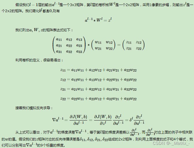
对于正向传播，我们使用原始的卷积核进行卷积操作。在反向传播时，为了计算输入或权重的梯度，通常需要进行“翻转”操作。

需要注意的是，正向卷积和反向传播中的卷积（通常称为转置卷积或反卷积）在数学和实现上有一些不同。在正向传播中，卷积核与输入数据进行卷积以生成输出。而在反向传播中，我们关心的是如何改变输入或卷积核以最小化某个损失函数。

为了具体说明为什么需要翻转卷积核，考虑一维情况（二维情况是类似的）：

假设正向卷积表示为 $y = x * w$ ，其中 $x$ 是输入， $w$ 是卷积核， $y$ 是输出，‘*’ 是卷积操作。

在反向传播过程中，我们通常需要计算损失函数 $L$ 关于输入 $x$ 的梯度（ $\frac{\partial L}{\partial x}$ ）。为了找到这个梯度，我们需要用到链式法则：

$\frac{\partial L}{\partial x} = \frac{\partial L}{\partial y} * \text{rot180}(w)$

其中， $\text{rot180}(w)$ 表示将 $w$ 进行180度翻转。

这样做的主要原因是数学上的一致性和计算的方便性。这样，前向和反向传播可以用相似的卷积操作来实现，大大简化了算法的实现。

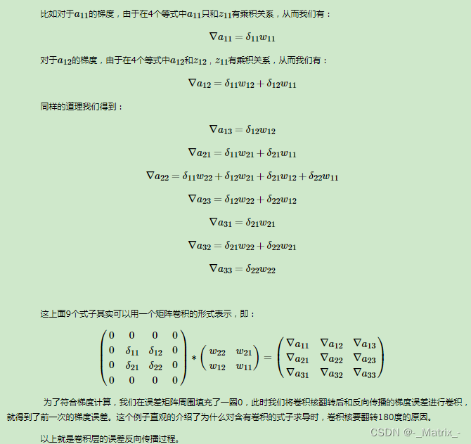
简而言之，在正向传播中我们使用原始的卷积核，而在反向传播时，为了计算梯度，我们通常需要用到翻转的卷积核。这主要是为了数学和计算的方便。

在反向传播（backpropagation）过程中，通常会使用原始卷积核（kernel）的翻转版本。这里的“翻转”通常意味着沿两个空间维度（即不是批量维度或通道维度）旋转180度。

例如，如果你有一个3x3的卷积核：

$\begin{pmatrix}a & b & c \\d & e & f \\g & h & i\end{pmatrix}$

翻转这个卷积核会得到：

$K^{\text{rot}} = \begin{pmatrix}i & h & g\\f & e & d \\c & b & a\end{pmatrix}$

在Eigen中，使用reverse()函数并指定需要翻转的维度可以实现这一点。例如，对于一个Eigen::MatrixXf对象kernel，你可以这样翻转它：

Eigen::MatrixXf rotated_kernel = kernel.reverse();

这里简单假设reverse()默认沿两个维度翻转矩阵。实际使用中，请确保你正确地翻转了维度。

这个翻转的卷积核（或旋转180度的卷积核）通常用于反向传播过程中，以计算相对于输入的梯度。这与前向传播中使用的卷积核是同一个卷积核，只是翻转了。

【卷积神经网络中的反向传播动画演示】
在这里插入图片描述

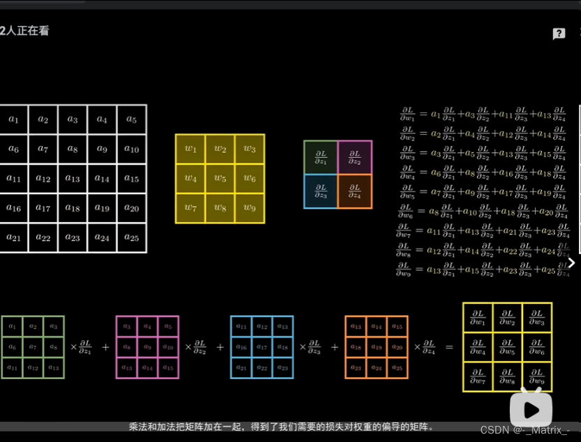
通过将输入和卷积核展开（unroll）为矩阵，可以使用矩阵乘法来实现卷积和转置卷积操作。下面简要介绍如何使用这种技术。

卷积

假设我们有一个输入矩阵 $X$ 和一个卷积核 $K$ 。我们首先将 $X$ 展开为一个大矩阵 $X_{\text{unroll}}$ ，其中每一列都包含一个 $K$ 能应用于 $X$ 的局部区域。然后，我们将 $K$ 展开为一个行向量 $K_{\text{unroll}}$ 。

接下来，卷积操作可以通过以下矩阵乘法进行：

$K_{\text{unroll}} \times X_{\text{unroll}}$

其中 $O$ 是输出矩阵。

转置卷积

对于转置卷积，方法基本相同，但展开和乘法的方向会有所不同。

假设我们有一个输入矩阵 $Y$ 和相同的卷积核 $K$ 。为了进行转置卷积，我们将 $Y$ 展开为 $Y_{\text{unroll}}$ ，然后执行以下矩阵乘法：

$X_{\text{unroll}} \times K^T$

这里， $K^T$ 是 $K$ 的转置。

请注意，在这两种情况下，我们都需要格外注意矩阵的维度和展开的顺序。

卷积核和反卷积的三种实现方式

#include <Eigen/Dense>
#include <iostream>

//卷积
Eigen::MatrixXf conv2D(const Eigen::MatrixXf& input, const Eigen::MatrixXf& kernel, int stride) {
    // 计算输出矩阵的尺寸
    int rows = (input.rows() - kernel.rows()) / stride + 1;
    int cols = (input.cols() - kernel.cols()) / stride + 1;

    // 创建输出矩阵
    Eigen::MatrixXf output(rows, cols);

    for (int i = 0; i < rows; ++i) {
        for (int j = 0; j < cols; ++j) {
            // 计算每个输出元素
            Eigen::MatrixXf block = input.block(i * stride, j * stride, kernel.rows(), kernel.cols());
            output(i, j) = (block.array() * kernel.array()).sum();
        }
    }
    return output;
}


// deconv2D 是一个函数，用于执行反卷积（也叫转置卷积）
Eigen::MatrixXf deconv2D( const Eigen::MatrixXf& y_grad,const Eigen::MatrixXf& kernel, int stride) {
    // 计算输出尺寸
    int outputRows = (y_grad.rows() - 1) * stride + kernel.rows();
    int outputCols = (y_grad.cols() - 1) * stride + kernel.cols();

    // 初始化输出矩阵为零
    Eigen::MatrixXf output = Eigen::MatrixXf::Zero(outputRows, outputCols);

    // 进行转置卷积操作
    for (int i = 0; i < y_grad.rows(); ++i) {
        for (int j = 0; j < y_grad.cols(); ++j) {
            // 注意：这里我们假设步长（stride）是1，你可以通过修改下面的索引来调整步长
            output.block(i * stride, j * stride, kernel.rows(), kernel.cols()) += y_grad(i, j) * kernel;
        }
    }

    return output;
}

// 转置卷积
Eigen::MatrixXf Conv2DTransposed( int rows,int cols ,const Eigen::MatrixXf& kernel, int stride)
{
    int r = (rows - kernel.rows()) / stride + 1;
    int c = (cols - kernel.cols()) / stride + 1;
    
    // 初始化输出矩阵为零
    Eigen::MatrixXf output1 = Eigen::MatrixXf::Zero(r * c, rows * cols);

    int jj =0;
    // 进行转置卷积操作
    for (int i = 0; i < r; ++i)
    {
        for (int j = 0; j < c ; ++j)
        {
            // 初始化输出矩阵为零
            Eigen::MatrixXf output = Eigen::MatrixXf::Zero(rows, cols);
            // 注意：这里我们假设步长（stride）是1，你可以通过修改下面的索引来调整步长
            output.block(i * stride, j * stride, kernel.rows(), kernel.cols()) = kernel;

            output1.row(jj++) = output.reshaped<Eigen::RowMajor>();
        }
    }

    return output1;
}
//图像转换为列
Eigen::MatrixXf im2col(const Eigen::MatrixXf& input, int kernel_rows, int kernel_cols, int stride) {
    int output_rows = (input.rows() - kernel_rows) / stride + 1;
    int output_cols = (input.cols() - kernel_cols) / stride + 1;

    Eigen::MatrixXf output(kernel_rows * kernel_cols, output_rows * output_cols);

    int col_idx = 0;
    for (int row = 0; row <= input.rows() - kernel_rows; row += stride)
    {
        for (int col = 0; col <= input.cols() - kernel_cols; col += stride)
        {
            Eigen::VectorXf col_vector = input.block(row, col, kernel_rows, kernel_cols).reshaped<Eigen::RowMajor>();
            //const Eigen::VectorXf col_vector = Eigen::Map<const Eigen::VectorXf, Eigen::RowMajor>(block.data(), block.size());
            output.col(col_idx++) = col_vector;
        }
    }
    return output;
}

//列转换为图像
Eigen::MatrixXf col2im(const Eigen::MatrixXf& input, int original_rows, int original_cols, int kernel_rows, int kernel_cols, int stride) {
    Eigen::MatrixXf output = Eigen::MatrixXf::Zero(original_rows, original_cols);

    int col_idx = 0;
    for (int row = 0; row <= original_rows - kernel_rows; row += stride)
    {
        for (int col = 0; col <= original_cols - kernel_cols; col += stride)
        {
            Eigen::MatrixXf block = input.col(col_idx++).reshaped<Eigen::RowMajor>(kernel_rows, kernel_cols);
            //const Eigen::MatrixXf block = Eigen::Map<const Eigen::MatrixXf, Eigen::RowMajor>(col_vector.data(), kernel_rows, kernel_cols);
            output.block(row, col, kernel_rows, kernel_cols) += block;
        }
    }

    return output;
}

int main() {
    // 用于测试的输入和卷积核
    Eigen::MatrixXf input(5, 5);
    input << 1, 2, 3, 4, 5,
            5, 4, 3, 2, 1,
            1, 2, 3, 4, 5,
            5, 4, 3, 2, 1,
            1, 2, 3, 4, 5;

    Eigen::MatrixXf kernel(3, 3);
    kernel << 1, 0, -1,
            1, 5, -1,
            1, 4, -1;

    int stride = 2;

    //第一种实现：正常卷积
    {
        //卷积
        Eigen::MatrixXf output = conv2D(input, kernel, stride);
        std::cout << "1: Conv2D Output:\n" << output << std::endl;
        //反卷积
        Eigen::MatrixXf output1 = deconv2D(output,kernel, stride);
        std::cout << "1: deconv2D output1:\n" << output1 << std::endl;
    }

    //第二种实现：转置卷积
    {
        Eigen::MatrixXf Unfold = Conv2DTransposed(input.rows(),input.cols(),kernel,stride);
        std::cout << "2: Unfold:\n" << Unfold << std::endl;
        Eigen::VectorXf Input = input.reshaped<Eigen::RowMajor>();
        Eigen::MatrixXf output = Unfold * Input;
        std::cout << "2: Conv2D Output:\n" << output << std::endl;

        Eigen::MatrixXf output1 =  (Unfold.transpose() * output).reshaped<Eigen::RowMajor>(input.rows(),input.cols());

        std::cout << "2: deconv2D output1:\n" << output1 << std::endl;
    }
     //第三种种实现：图像转换为列  矩阵相乘实现  加速运算
    {
        Eigen::MatrixXf input_unroll = im2col(input, kernel.rows(),kernel.cols(), stride);
        Eigen::RowVectorXf kernel_unroll = kernel.reshaped<Eigen::RowMajor>();
        Eigen::MatrixXf output = kernel_unroll * input_unroll ;
        std::cout << "3: Conv2D Output:\n" << output << std::endl;

        Eigen::MatrixXf output_unroll11 = kernel_unroll.transpose() * output;
        std::cout << "3: output_unroll11:\n" << output_unroll11 << std::endl;

        Eigen::MatrixXf output1 = col2im(output_unroll11, input.rows(),input.cols(),kernel.rows(),kernel.cols(), stride);
        std::cout << "3: deconv2D output1:\n" << output1 << std::endl;

    }

}

1: Conv2D Output:
26 24
26 24
1: deconv2D output1:
 26   0  -2   0 -24
 26 130  -2 120 -24
 52 104  -4  96 -48
 26 130  -2 120 -24
 26 104  -2  96 -24
2: Unfold:
 1  0 -1  0  0  1  5 -1  0  0  1  4 -1  0  0  0  0  0  0  0  0  0  0  0  0
 0  0  1  0 -1  0  0  1  5 -1  0  0  1  4 -1  0  0  0  0  0  0  0  0  0  0
 0  0  0  0  0  0  0  0  0  0  1  0 -1  0  0  1  5 -1  0  0  1  4 -1  0  0
 0  0  0  0  0  0  0  0  0  0  0  0  1  0 -1  0  0  1  5 -1  0  0  1  4 -1
2: Conv2D Output:
26
24
26
24
2: deconv2D output1:
 26   0  -2   0 -24
 26 130  -2 120 -24
 52 104  -4  96 -48
 26 130  -2 120 -24
 26 104  -2  96 -24
3: Conv2D Output:
26 24 26 24
3: output_unroll11:
 26  24  26  24
  0   0   0   0
-26 -24 -26 -24
 26  24  26  24
130 120 130 120
-26 -24 -26 -24
 26  24  26  24
104  96 104  96
-26 -24 -26 -24
3: deconv2D output1:
 26   0  -2   0 -24
 26 130  -2 120 -24
 52 104  -4  96 -48
 26 130  -2 120 -24
 26 104  -2  96 -24

卷积的次数计算

在这里插入图片描述

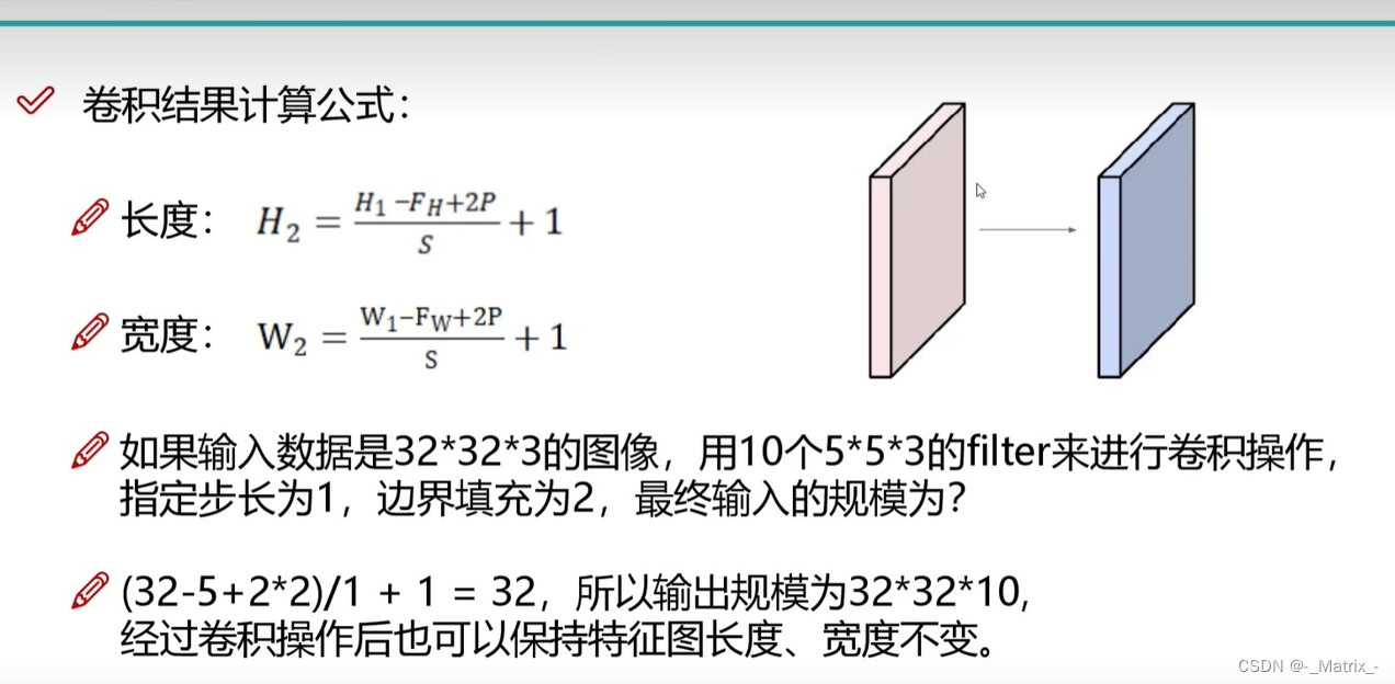
当然可以。给定一个输入特征图的大小和一个滤波器的大小，以及卷积的步长和填充，以下是如何计算卷积后的输出特征图的维度的完整公式：

高度 $H_2$ 的计算：
$H_2 = \frac{H_1 - F_{H} + 2P}{S} + 1$
宽度 $W_2$ 的计算：
$W_2 = \frac{W_1 - F_{W} + 2P}{S} + 1$

其中：

$H_1, W_1$ 是输入特征图的高和宽。
$F_H, F_W$ 是滤波器的高和宽。
$P$ 是填充的数量。
$S$ 是步长。

以下是使用C++和Eigen库实现的示例：

#include <Eigen/Dense>
#include <iostream>
#include <cmath>

std::pair<int, int> computeConvTimes(int input_rows, int input_cols, int kernel_rows, int kernel_cols, int stride) {
    int rows_times = (input_rows - kernel_rows) / stride + 1;
    int cols_times = (input_cols - kernel_cols) / stride + 1;
    
    return {rows_times, cols_times};
}

int main() {
    int input_rows = 5, input_cols = 5;
    int kernel_rows = 3, kernel_cols = 3;
    int stride = 2;

    auto [rows_times, cols_times] = computeConvTimes(input_rows, input_cols, kernel_rows, kernel_cols, stride);

    std::cout << "Rows can be convolved: " << rows_times << " times.\n";
    std::cout << "Columns can be convolved: " << cols_times << " times.\n";

    return 0;
}

这段代码首先定义了一个函数computeConvTimes，该函数使用上述公式计算行和列的卷积次数。然后在main函数中展示了对于给定的输入大小、核大小和步长，可以进行多少次卷积操作。

-_Matrix_-

关注

28
点赞
踩
27

收藏

觉得还不错? 一键收藏
0
评论
神经网络系列---卷积

需要注意的是，正向卷积和反向传播中的卷积（通常称为转置卷积或反卷积）在数学和实现上有一些不同。在神经网络的卷积层中，向下取整（Floor）是一种常用的策略，特别是在处理输出尺寸不是整数的情况时。这个翻转的卷积核（或旋转180度的卷积核）通常用于反向传播过程中，以计算相对于输入的梯度。简而言之，在正向传播中我们使用原始的卷积核，而在反向传播时，为了计算梯度，我们通常需要用到翻转的卷积核。对于正向传播，我们使用原始的卷积核进行卷积操作。举一个简单的例子，假设你有一个7x7的输入和一个3x3的卷积核，步长为2。
复制链接

扫一扫