线性回归算法从0开始的实现

参考：

range函数作用
sum（）函数作用
backward作用
torch.matmul()用法介绍
yield作用
with语法
grad作用

各模块分析

构造数据集

我们是构造已知W，b的具体数据

• num_examples为生成的样本数
• torch.matmul()用法介绍
• torch.normal生成均值为0，方差为1，大小为W的长度的n各样本的随机数
• y.reshape((-1, 1)的作用为转化y的形状

#构造人造数据集
def synthetic_data(w, b, num_examples):  #@save
    """生成y=Xw+b+噪声"""
    #生成一个均值为0，方差为1的随机数X，
    # 大小为n个样本，列数为w的长度
    X = torch.normal(0, 1, (num_examples, len(w)))
    y = torch.matmul(X, w) + b
    #加入一个均值为0，方差为0.01，形状为y同样形状的噪音
    y += torch.normal(0, 0.01, y.shape)
   #print("X.shape==",X.shape,"y.shape==",y.shape)
    return X, y.reshape((-1, 1))

true_w = torch.tensor([2, -3.4])
true_b = 4.2
features, labels = synthetic_data(true_w, true_b, 1000)
print('features:', features[0],'\nlabel:', labels[0])

我们可以输出查看X，y的形状

print("X.shape==",X.shape,"y.shape==",y.shape)
>>>X.shape== torch.Size([1000, 2]) y.shape== torch.Size([1000])

读取小批量数据

• 每次读入batch_size长度的数据
• features, labels分别为synthetic_data构造数据集中返回的X，y.reshape
• yield作用，相当于一个下一次返回地点是上一次结束地点的return

def data_iter(batch_size, features, labels):
    num_examples = len(features)
    #生成每个样本的列表数据
    indices = list(range(num_examples))
    # 这些样本是随机读取的，没有特定的顺序
    #使用random.shuffle将下标完全打乱，随机打乱后用随机顺序访问样本
    random.shuffle(indices)  print("num+examples:",num_examples,'\nbatch_size:',batch_size)
    
    #产生从0到num_examples，每一次跳batch_size的大小
    for i in range(0, num_examples, batch_size):
    #min的在作用是防止最后一次取值不能取满，所有如果没有取满，就用num_examples
        batch_indices = torch.tensor(
            indices[i: min(i + batch_size, num_examples)])
        
        yield features[batch_indices], labels[batch_indices]
#生成batch_size的小批量
batch_size = 10

for X, y in data_iter(batch_size, features, labels):
    print('X==',X, '\ny==', y)
    break

对for循环中的数据进行检查如下

num_examples: 1000 
batch_size: 10
i== 0 batch_indices== tensor([499, 440, 731, 154, 335, 898, 874, 842, 238, 969])
i== 10 batch_indices== tensor([ 12, 794, 745, 243, 780, 357, 379, 405, 669, 551])
i== 20 batch_indices== tensor([218, 309, 565, 839, 858, 579, 718, 818, 429, 519])
i== 30 batch_indices== tensor([726, 988, 475, 531, 829,   3, 580, 658, 948, 861])
......
i== 980 batch_indices== tensor([127, 623,  95, 553, 156, 474, 947, 884, 518, 997])
i== 990 batch_indices== tensor([935, 200, 267, 472, 782, 351, 674,  48, 632, 511])

初始化模型参数

w = torch.normal(0, 0.01, size=(2,1), requires_grad=True)
b = torch.zeros(1, requires_grad=True)
print('\n\nw==',w,'\nb==',b)

w== tensor([[-0.0048]，[-0.0116]],requires_grad=True) 
b== tensor([0.], requires_grad=True)

线性回归模型函数

线性回归模型原理

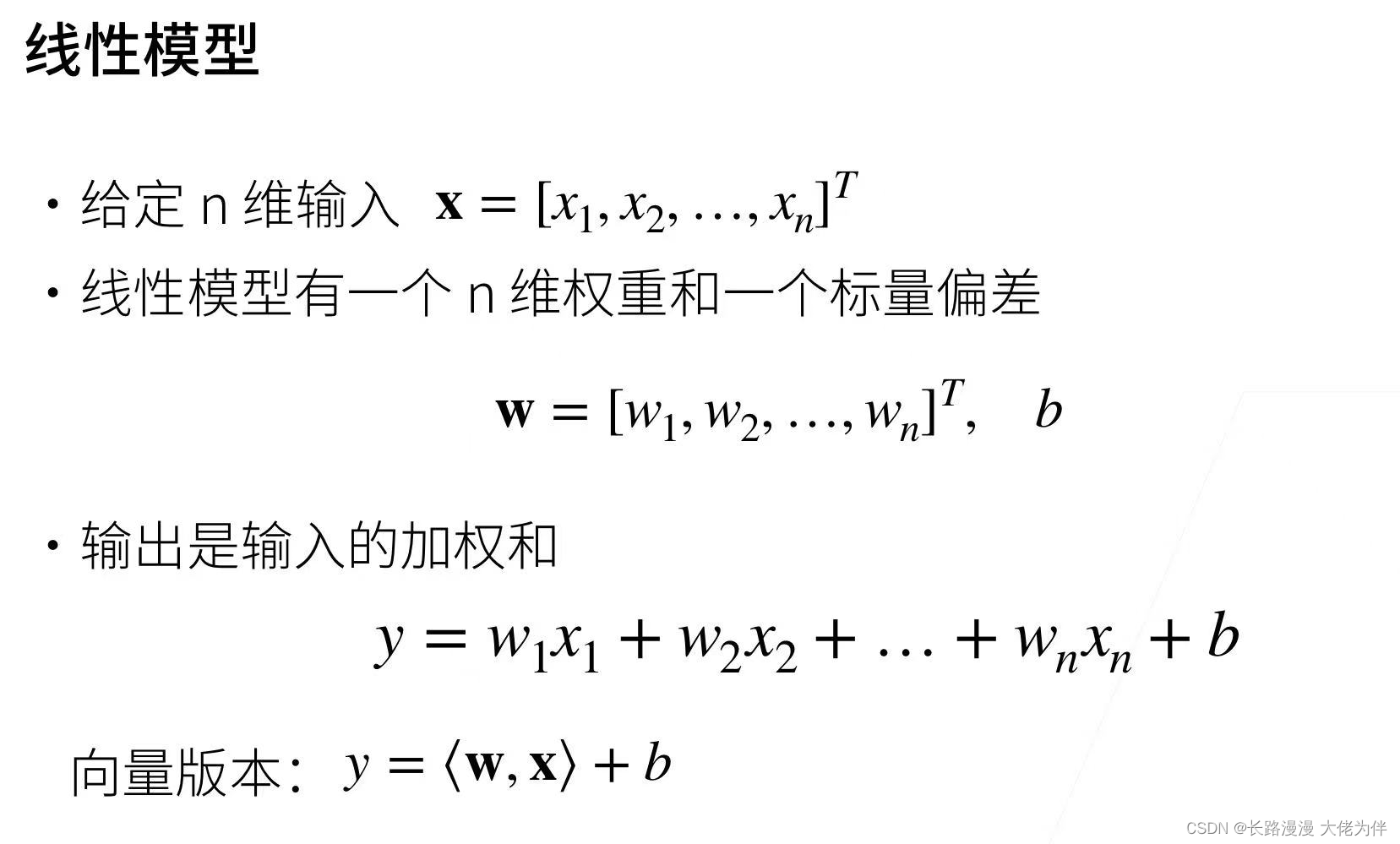
线性回归模型实现

torch.matmul()用法介绍

def linreg(X, w, b):  
    """线性回归模型。"""
    return torch.matmul(X, w) + b

其中可以看出torch.matmul(X, w)的形状

print(torch.matmul(X, w).shape)
torch.Size([1000, 1])

均方损失模型

均方损失模型原理

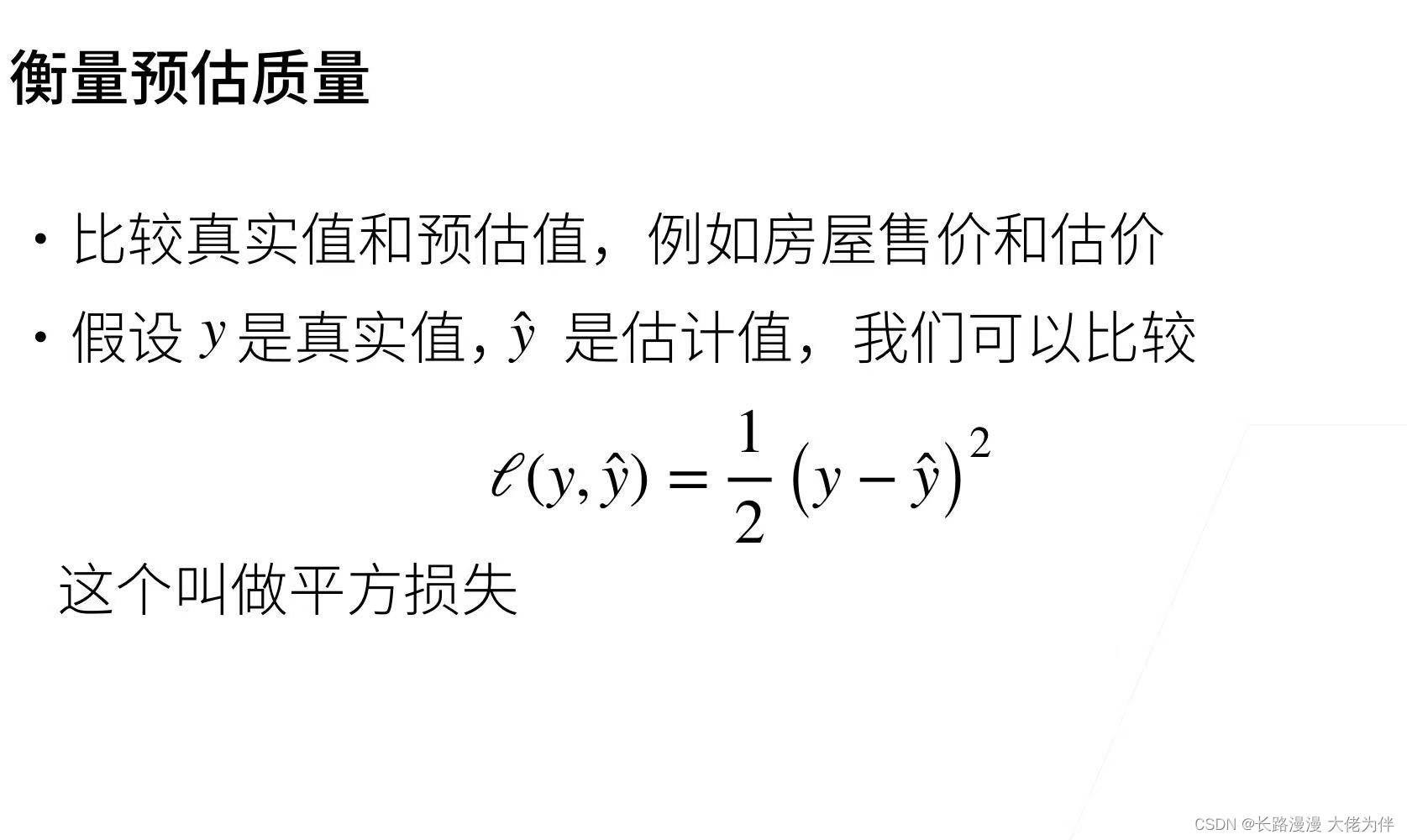
均方损失模型实现

def squared_loss(y_hat, y):  #@save
    """均方损失"""
    return (y_hat - y.reshape(y_hat.shape)) ** 2 / 2

其中y_hat为真实值

y.reshape(y_hat.shape)

因为y与y_hat的元素个数可能是一样，但是可能会一个是向量，一个是行向量或者列向量，所以将y和y_hat的维度统一，方便进行计算

定义优化算法

优化算法原理

通过对初始值的迭代，按学习率沿梯度方向逐步求最优值

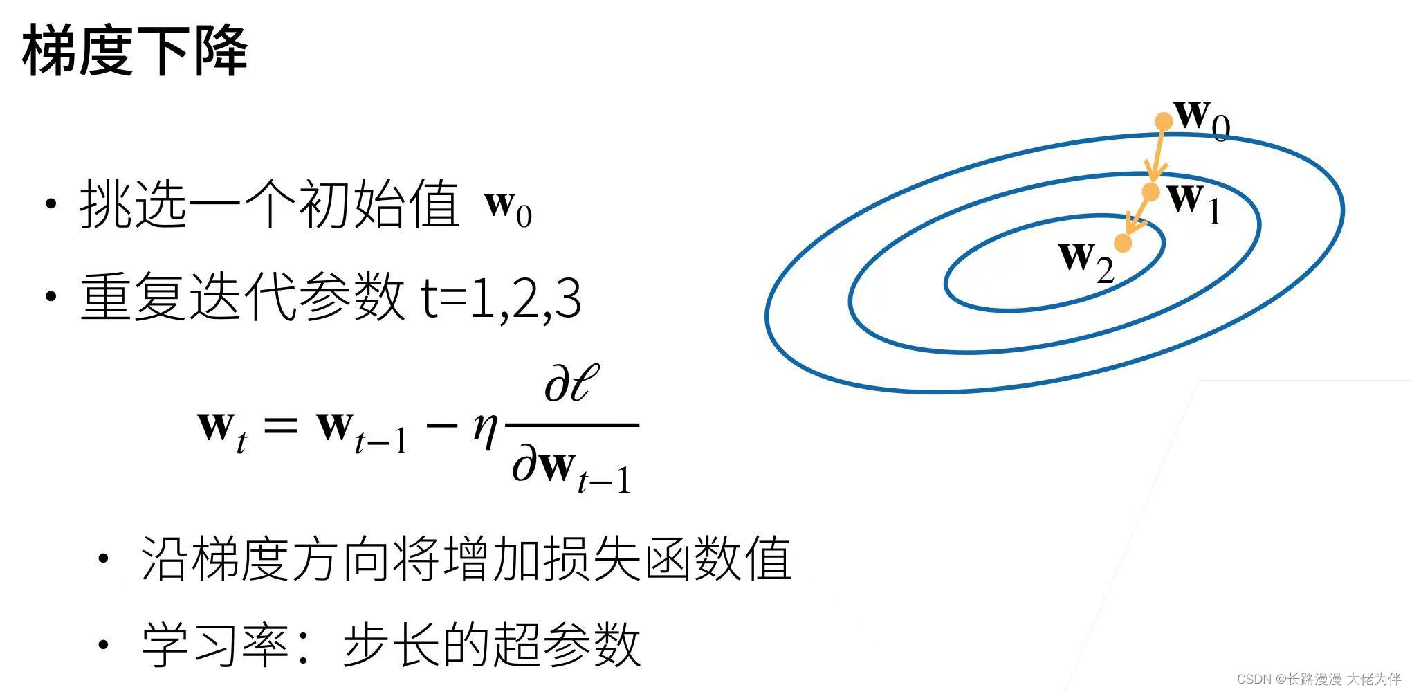
优化算法实现

def sgd(params, lr, batch_size):  #@save
    """小批量随机梯度下降"""
    with torch.no_grad():
        for param in params:
            param -= lr * param.grad / batch_size
            param.grad.zero_()

param -= lr * param.grad / batch_size

grad作用，用来求导

param.grad.zero_()

pytorch中不会对梯度自动设为0，这里需要人为设置

最终实现

先来看看调用实现，

• 将学习率设为lr
• 梯度更新次数为3次
• linreg函数为定义线性回归模型的函数
• squared_loss函数为损失函数
• data_iter函数作用为读取小批量数据
• sgd函数作用为更新梯度

l.sum().backward()

• sum的作用，将向量转化为标量，因为backward是对标量进行处理，backward只能被应用在一个标量上，也就是一个一维tensor
• backward作用：对标量自动求导

lr = 0.03
num_epochs = 3
net = linreg
loss = squared_loss
for epoch in range(num_epochs):
    for X, y in data_iter(batch_size, features, labels):
        l = loss(net(X, w, b), y)  # X和y的小批量损失
        # 因为l形状是(batch_size,1)，而不是一个标量。l中的所有元素被加到一起，
        # 并以此计算关于[w,b]的梯度
        l.sum().backward()
        sgd([w, b], lr, batch_size)  # 使用参数的梯度更新参数
    with torch.no_grad():
        train_l = loss(net(features, w, b), labels)
        print(f'epoch {epoch + 1}, loss {float(train_l.mean()):f}')

print(f'w的估计误差: {true_w - w.reshape(true_w.shape)}')
print(f'b的估计误差: {true_b - b}')

运行结果：

epoch 1, loss 0.042265
epoch 2, loss 0.000164
epoch 3, loss 0.000053
w的估计误差: tensor([ 0.0006, -0.0007], grad_fn=<SubBackward0>)
b的估计误差: tensor([0.0002], grad_fn=<RsubBackward1>)