diffusion_S example简单易懂

%matplotlib inline
import matplotlib.pyplot as plt
import numpy as np
from sklearn.datasets import make_s_curve
import torch

1. 生成数据

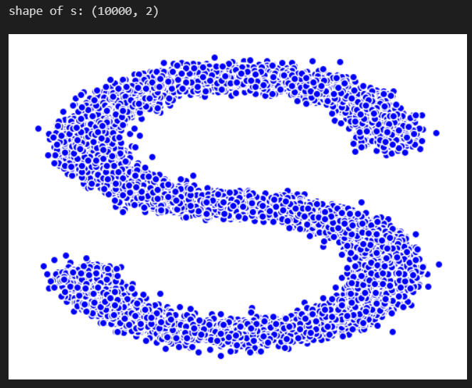
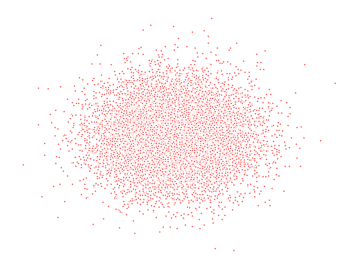
s_curve,_ = make_s_curve(10**4,noise=0.1)# 1万个点
print(_.shape)
print(s_curve[0])#点的三维坐标，(x,y,z)
# print(s_curve[0].T)
# https://scikit-learn.org/stable/auto_examples/manifold/plot_compare_methods.html#sphx-glr-auto-examples-manifold-plot-compare-methods-py
# https://blog.csdn.net/weixin_42887138/article/details/117656280
print(_[0])  # 点的颜色值

# 画出数据集的形状
s_curve,_ = make_s_curve(10**4,noise=0.1)#  产生1万个样本点，3维的(x,y,z)
s_curve = s_curve[:,[0,2]]/10.0   #取出(x,z)然后画出2维的S图

print("shape of s:",np.shape(s_curve))

data = s_curve.T
# data=s_curve

fig,ax = plt.subplots() # https://blog.csdn.net/htuhxf/article/details/82986440
ax.scatter(*data,color='blue',edgecolor='white');

ax.axis('off')

dataset = torch.Tensor(s_curve).float()  
# 张量也可以写成dataset的，dataset不一定要写为class，当数据比较简单的时候，我们可以直接写成张量的形式

2. 确定超参数的值

num_steps = 100    # 即T,对于步骤，一开始可以由beta, 分布的均值和标准差来共同确定

#制定每一步的beta
betas = torch.linspace(-6,6,num_steps)     # size:100
betas = torch.sigmoid(betas)*(0.5e-2 - 1e-5)+1e-5   
# beta是递增的，最小值为0.00001,最大值为0.005, sigmooid func
# 像学习率一样的一个东西，而且是一个比较小的值，所以就有理由假设逆扩散过程也是一个高斯分布

#计算alpha、alpha_prod、alpha_prod_previous、alpha_bar_sqrt等变量的值
alphas = 1-betas    # size: 100
alphas_prod = torch.cumprod(alphas,0)    # size: 100
# 就是让每一个都错一下位
alphas_prod_p = torch.cat([torch.tensor([1]).float(),alphas_prod[:-1]],0)  # p表示previous  
# alphas_prod[:-1] 表示取出 从0开始到倒数第二个值
alphas_bar_sqrt = torch.sqrt(alphas_prod)
one_minus_alphas_bar_log = torch.log(1 - alphas_prod)
one_minus_alphas_bar_sqrt = torch.sqrt(1 - alphas_prod)

assert alphas.shape==alphas_prod.shape==alphas_prod_p.shape==\
alphas_bar_sqrt.shape==one_minus_alphas_bar_log.shape\
==one_minus_alphas_bar_sqrt.shape
print("all the same shape",betas.shape)
# 每一时刻这些量的值都是不一样的，但是他们是不需要训练的，是超参数

3. 确定扩散过程任意时刻的采样值

$q(x_t|x_0)=N(x_t;\sqrt{{\bar{\alpha }}_t}{x}_0,(1-{\bar{\alpha }}_t)I)$
即给定初始的$x_0$的分布就可以求出任意时刻$x_t$的采样值

$\mu =\sqrt{{\bar{\alpha }}_t}{x}_0,\sigma =\sqrt{1-{\bar{\alpha }}_t}$
noise:$ϵ$
$x_0=ϵ\ast \sigma +\mu$

#计算任意时刻的x采样值，基于x_0和重参数化
def q_x(x_0,t):
    """可以基于x[0]得到任意时刻t的x[t]"""

    noise = torch.randn_like(x_0)   # noise是从正态分布中生成的随机噪声
    alphas_t = alphas_bar_sqrt[t]
    alphas_1_m_t = one_minus_alphas_bar_sqrt[t]
    return (alphas_t * x_0 + alphas_1_m_t * noise)#在x[0]的基础上添加噪声

# 上面就可以通过x0和t来采样出xt的值

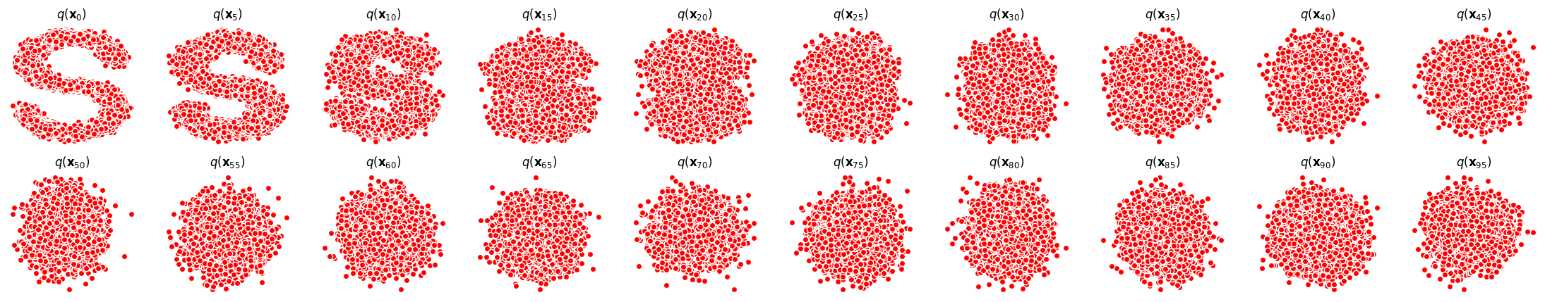
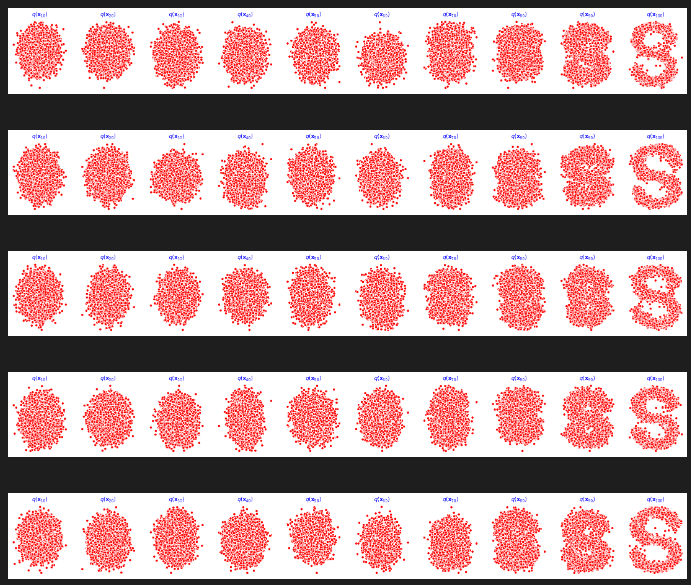
4. 演示原始数据分布加噪100步后的结果

num_shows = 20
fig,axs = plt.subplots(2,10,figsize=(28,5))
plt.rc('text',color='black')

#共有10000个点，每个点包含两个坐标
#生成100步以内每隔5步加噪声后的图像
for i in range(num_shows):
    j = i//10
    k = i%10
    # 每一时刻的点都是基于q(xt|x0)采样得到的
    q_i = q_x(dataset,torch.tensor([i*num_steps//num_shows]))#生成t时刻的采样数据, //表示地板除，先做除法，再向下取整
    axs[j,k].scatter(q_i[:,0],q_i[:,1],color='red',edgecolor='white')
    axs[j,k].set_axis_off()
    axs[j,k].set_title('$q(\mathbf{x}_{'+str(i*num_steps//num_shows)+'})$')


# forward diffusion process 不含参数

5. 编写拟合逆扩散过程高斯分布的模型

对应于$L_{simple(\theta )}$中的${ϵ}_{\theta }(\sqrt{{\bar{\alpha }}_t}{x}_0+\sqrt{1-{\bar{\alpha }}_t}ϵ,t)$, 左式以$x_0,t$作为输入，输出是与$x_0$的形状一致的一个网络,因为${ϵ}_{\theta }$就是要去逼近$ϵ$,而$ϵ$是与$x_0$的形状一致
下面MLPDiffusion中forward(self, x,t)中的x其实指的是$\sqrt{{\bar{\alpha }}_t}{x}_0+\sqrt{1-{\bar{\alpha }}_t}ϵ$

import torch
import torch.nn as nn

class MLPDiffusion(nn.Module):
    def __init__(self,n_steps,num_units=128):
        super(MLPDiffusion,self).__init__()
        
        # https://blog.csdn.net/weixin_36670529/article/details/105910767
        # 它和torch的其他机制结合紧密，继承了nn.Module的网络模型class可以使用nn.ModuleList并识别其中的parameters，当然这只是个list，不会自动实现forward方法。可见，
        # 普通list中的子module并不能被主module所识别，而ModuleList中的子module能够被主module所识别
        # nn.Sequential定义的网络中各层会按照定义的顺序进行级联，需要保证各层的输入和输出之间要衔接
        # nn.Sequential实现了forward()方法，因此可以直接通过x = self.combine(x)的方式实现forward
        # 而nn.ModuleList则没有顺序性要求，也没有forward()方法
        self.linears = nn.ModuleList(
            [
                nn.Linear(2,num_units),
                nn.ReLU(),
                nn.Linear(num_units,num_units),
                nn.ReLU(),
                nn.Linear(num_units,num_units),
                nn.ReLU(),
                nn.Linear(num_units,2),  # input shape = output shape = 2
            ]
        )
        # https://pytorch.org/docs/stable/generated/torch.nn.Embedding.html
        self.step_embeddings = nn.ModuleList(
            [
                nn.Embedding(n_steps,num_units),   # 一个字典中有100个词，每个词嵌入向量的大小为128 dim
                nn.Embedding(n_steps,num_units),
                nn.Embedding(n_steps,num_units), # n_step=T=100步，num_units即hidden layer的parameter 
            ]
        )
    def forward(self,x,t):
        # 训练的时候不是按顺序给的，是随机采样的，需要额外的时间信息
        # 也可以不用embedding,直接送T进去训练，但这种信息无法很好学到，embedding层会嵌入时间的信息，变成网络更容易理解的模式。
        # transformer也是这样加时间信息的
        # x = x_0
        for idx,embedding_layer in enumerate(self.step_embeddings):
            t_embedding = embedding_layer(t)   # 把t编码为128维的embedding
            x = self.linears[2*idx](x)   # linear
            x += t_embedding    # embedding是通过加法加进去的
            x = self.linears[2*idx+1](x) # relu
            
        x = self.linears[-1](x) # linear，保证x的形状不变
        
        return x

6. 编写训练的误差函数

$L_{simple}(\theta ):={\mathbb{E}}_{t,x_0,ϵ}\left[||ϵ-{ϵ}_{\theta }(\sqrt{{\bar{\alpha }}_t}{x}_0+\sqrt{1-{\bar{\alpha }}_t}ϵ,t)|{|}^2\right]$

model: 算出${ϵ}_{\theta }$
n_steps:算loss时，从时间范围内随机生成一些t

model:输入的其实是$x_t,t$, 这个$x_t$是通过前向扩散过程 $x_0$ 和 $ϵ$ 计算出来的,即$x_t=\sqrt{\bar{\alpha }}{x}_0+\sqrt{1-{\bar{\alpha }}_t}ϵ$
，再输入到model中的, 得到 ${ϵ}_{\theta }$

注意：
diffusion_loss_fn中的时间t 序列，并不是按顺序从$1,2,3,...t$，而是随机生成一系列的时刻t,因为$x_t$可以直接由$x_0$和t计算出来，所以其实在训练的过程中我们并不需要马尔科夫链的过程，一步就求出t时刻的$x_t$了。

def diffusion_loss_fn(model, x_0, alphas_bar_sqrt, one_minus_alphas_bar_sqrt, n_steps):
    """对任意时刻t进行采样计算loss"""
    batch_size = x_0.shape[0]
    # n_steps是为了算loss的时候，可以在n_steps这个范围内随机地生成一些t
    
    #对一个batchsize样本生成随机的时刻t,覆盖到更多不同的t
    t = torch.randint(0,n_steps,size=(batch_size//2,))  #  size=(batch_size//2,)中的,不可少
    t = torch.cat([t,n_steps-1-t],dim=0)# [batchsize]
    t = t.unsqueeze(-1)#[batchsize, 1]
    
    #x0的系数
    a = alphas_bar_sqrt[t]
    
    #eps的系数
    aml = one_minus_alphas_bar_sqrt[t]
    
    #生成随机噪音eps
    e = torch.randn_like(x_0)
    
    #构造模型的输入,即x_t可以用x_0和t来表示
    x = x_0*a+e*aml
    
    #送入模型，得到t时刻的随机噪声预测值
    output = model(x,t.squeeze(-1))
    
    #与真实噪声一起计算误差，求平均值
    return (e - output).square().mean()
    # 目的：让网络预测的噪声  接近于  真实扩散过程的噪声

7. 编写逆扩散采样函数（inference过程）

${\mu }_{\theta }({\mathbf{x}}_t,t)=\stackrel{\sim }{{\mu }_t}\left({\mathbf{x}}_t,\frac{1}{\sqrt{{\bar{\alpha }}_t}}({\mathbf{x}}_t-\sqrt{1-{\bar{\alpha }}_t}.{ϵ}_{\theta }({\mathbf{x}}_t))\right)=\frac{1}{\sqrt{{\alpha }_t}}\left({\mathbf{x}}_t-\frac{{\beta }_t}{\sqrt{1-{\bar{\alpha }}_t}}.{ϵ}_{\theta }({\mathbf{x}}_t,t)\right)$
里面的${ϵ}_{\theta }$是通过模型算出来的，就是说这个模型的输出是 ${ϵ}_{\theta }$
即下面函数p_sample中的mean
$p_{\theta }({\mathrm{x}}_{\mathrm{t}-1}|{\mathrm{x}}_{\mathrm{t}})=\mathcal{N}({\mathrm{x}}_{\mathrm{t}-1};{\mu }_{\theta }({\mathrm{x}}_{\mathrm{t}},\mathrm{t}),{\Sigma }_{\theta }(x_t,t))$,在论文中将其方差 ${\Sigma }_{\theta }(x_t,t)$ 设置程一个与 $\beta$ 相关的常数${\sigma }_t^{2}I$,且有${\sigma }_t^2=\stackrel{\sim }{{\beta }_t}=\frac{1-{\bar{\alpha }}_{t-1}}{1-{\bar{\alpha }}_t}{\beta }_t$
即$p_{\theta }(x_{t-1}|x_t)=\mathcal{N}(x_{t-1};{\mu }_{\theta }(x_t,t),{\sigma }_t^{2}I)$
$----------$
但是下面的好像直接设置${\sigma }_t^{2}I$,且有${\sigma }_t^2={\beta }_t$

上面方差的两种设置都可以，他们都不含参数

Algorithm 2 Sampling
${\mathbf{x}}_T\sim N(0,I)$
${\mathbf{x}}_{t-1}=\frac{1}{\sqrt{{\alpha }_t}}({\mathbf{x}}_t-\frac{1-{\alpha }_t}{\sqrt{1-{\bar{\alpha }}_t}}.{ϵ}_{\theta }({\mathbf{x}}_t,t))+{\sigma }_t\mathbf{z}$
其中，${ϵ}_{\theta }$是model预测出来的

总结：
p_sample: 即逆扩散过程的时候才用到，由 ${\mathbf{x}}_t$ 推出 ${\mathbf{x}}_{t-1}$, ${ϵ}_{\theta }$是由model预测出来的
p_sample_loop: 从标准分布的噪声 ${\mathbf{x}}_T$ 出发, 逆扩散过程是自回归的，即必须按顺序依次推出${\mathbf{x}}_t,{\mathbf{x}}_{t-1},{\mathbf{x}}_{t-2},\cdots ,{\mathbf{x}}_0$，不能并行inference

def p_sample_loop(model,shape,n_steps,betas,one_minus_alphas_bar_sqrt):
    """从x[T]恢复x[T-1]、x[T-2]|...x[0]"""
    cur_x = torch.randn(shape)  
    x_seq = [cur_x]
    for i in reversed(range(n_steps)):
   		# 逆扩散过程是自回归的，即必须按顺序依次推出x[t],x[t-1],x[t-2]...
        # 不能并行inference
        cur_x = p_sample(model,cur_x,i,betas,one_minus_alphas_bar_sqrt)
        x_seq.append(cur_x)
    # 把很多步采样拼起来
    return x_seq

def p_sample(model,x,t,betas,one_minus_alphas_bar_sqrt): # 参数重整化的过程
    """从x[t]采样t-1时刻的重构值，即从x[t]采样出x[t-1]"""
    t = torch.tensor([t])
    
    coeff = betas[t] / one_minus_alphas_bar_sqrt[t]
    
    eps_theta = model(x,t)
    
    mean = (1/(1-betas[t]).sqrt())*(x-(coeff*eps_theta))
    
    # 得到mean后，再生成一个随机量z，
    z = torch.randn_like(x)
    sigma_t = betas[t].sqrt()
    
    sample = mean + sigma_t * z
    # 上面就单步采样
    return (sample)

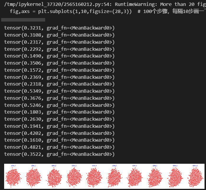
8. 开始训练模型，打印loss及中间重构效果

seed = 1234

class EMA():
    """构建一个参数平滑器"""
    def __init__(self,mu=0.01):
        self.mu = mu
        self.shadow = {}
        
    def register(self,name,val):
        self.shadow[name] = val.clone()
        
    def __call__(self,name,x):
        assert name in self.shadow
        new_average = self.mu * x + (1.0-self.mu)*self.shadow[name]
        self.shadow[name] = new_average.clone()
        return new_average
    
print('Training model...')
'''
ema = EMA(0.5)
for name, param in model.named_parameters():
    if param.requires_grad:
        ema.register(name, param.data)
'''


batch_size = 128
# 把dataset放入DataLoader中，构成一个dataloader
dataloader = torch.utils.data.DataLoader(dataset,batch_size=batch_size,shuffle=True)
num_epoch = 4000
plt.rc('text',color='blue')

model = MLPDiffusion(num_steps)#输出维度是2，输入是x和step,  num_steps=100
optimizer = torch.optim.Adam(model.parameters(),lr=1e-3)

for t in range(num_epoch):
    for idx,batch_x in enumerate(dataloader):

        loss = diffusion_loss_fn(model,batch_x,alphas_bar_sqrt,one_minus_alphas_bar_sqrt,num_steps)
        optimizer.zero_grad()
        loss.backward()
        # 对梯度进行clip ， 保证稳定性.
        # 当神经网络深度逐渐增加，网络参数量增多的时候，反向传播过程中链式法则里的梯度连乘项数便会增多，
        # 更易引起梯度消失和梯度爆炸。对于梯度爆炸问题，解决方法之一便是进行梯度剪裁，即设置一个梯度大小的上限。

        # 梯度裁剪应该放在loss.backward()和optimizer.step()之间
        # https://zhuanlan.zhihu.com/p/557949443
        torch.nn.utils.clip_grad_norm_(model.parameters(),1.)
        optimizer.step()
        # ema会导致在这个s的数据集上训练速度变慢，所以不用ema
        # for name, param in model.named_parameters():
        #     if param.requires_grad:
        #         param.data = ema(name, param.data)
        
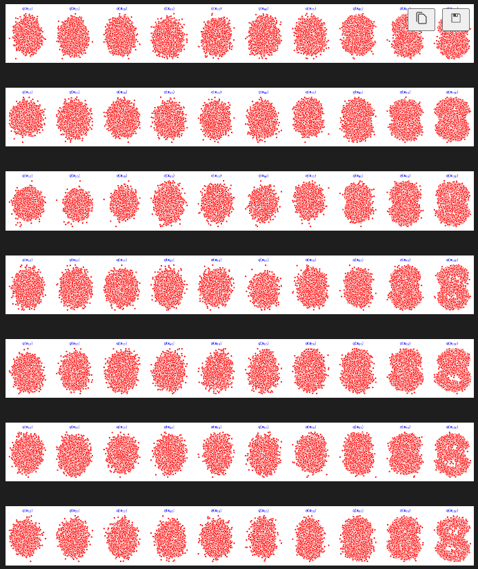
    if(t%100==0):
        print(loss)
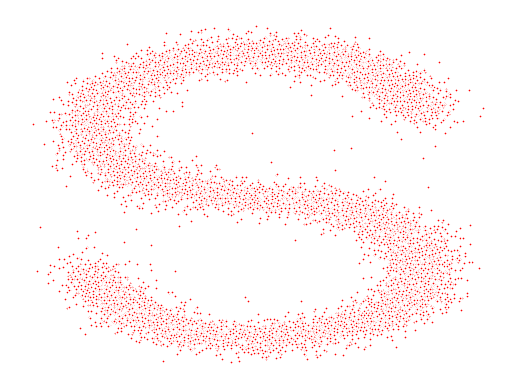
        x_seq = p_sample_loop(model,dataset.shape,num_steps,betas,one_minus_alphas_bar_sqrt) # 共有10个元素
        
        fig,axs = plt.subplots(1,10,figsize=(28,3))  # 100个步骤，每隔10步画一下
        # 每一行就代表了我们进行了100步的逆扩散的采样
        for i in range(1,11):
            cur_x = x_seq[i*10].detach()
            axs[i-1].scatter(cur_x[:,0],cur_x[:,1],color='red',edgecolor='white');
            axs[i-1].set_axis_off();
            axs[i-1].set_title('$q(\mathbf{x}_{'+str(i*10)+'})$')

9. 动画演示扩散过程和逆扩散过程

# Generating the forward image sequence  生成前向过程，也就是逐步加噪声

import io
from PIL import Image

imgs = []
for i in range(100):
    plt.clf()
    q_i = q_x(dataset,torch.tensor([i]))
    plt.scatter(q_i[:,0],q_i[:,1],color='red',edgecolor='white',s=5);
    plt.axis('off');
    
    img_buf = io.BytesIO()
    plt.savefig(img_buf,format='png')
    img = Image.open(img_buf)
    imgs.append(img)

reverse = []
for i in range(100):
    plt.clf()
    cur_x = x_seq[i].detach()
    plt.scatter(cur_x[:,0],cur_x[:,1],color='red',edgecolor='white',s=5);
    plt.axis('off')
    
    img_buf = io.BytesIO()
    plt.savefig(img_buf,format='png')
    img = Image.open(img_buf)
    reverse.append(img)

imgs = imgs +reverse

将前向的加噪声和后向的去噪结合起来生成gif

imgs[0].save("diffusion.gif",format='GIF',append_images=imgs,save_all=True,duration=100,loop=0)