


单变量线性回归
题目
在本部分的练习中,您将使用一个变量实现线性回归,以预测食品卡车的利润。假设你是一家餐馆的首席执行官,正在考虑不同的城市开设一个新的分店。该连锁店已经在各个城市拥有卡车,而且你有来自城市的利润和人口数据。
您希望使用这些数据来帮助您选择将哪个城市扩展到下一个城市。
数据
6.1101,17.592
5.5277,9.1302
8.5186,13.662
7.0032,11.854
5.8598,6.8233
8.3829,11.886
7.4764,4.3483
8.5781,12
6.4862,6.5987
5.0546,3.8166
5.7107,3.2522
14.164,15.505
5.734,3.1551
8.4084,7.2258
5.6407,0.71618
5.3794,3.5129
6.3654,5.3048
5.1301,0.56077
6.4296,3.6518
7.0708,5.3893
6.1891,3.1386
20.27,21.767
5.4901,4.263
6.3261,5.1875
5.5649,3.0825
18.945,22.638
12.828,13.501
10.957,7.0467
13.176,14.692
22.203,24.147
5.2524,-1.22
6.5894,5.9966
9.2482,12.134
5.8918,1.8495
8.2111,6.5426
7.9334,4.5623
8.0959,4.1164
5.6063,3.3928
12.836,10.117
6.3534,5.4974
5.4069,0.55657
6.8825,3.9115
11.708,5.3854
5.7737,2.4406
7.8247,6.7318
7.0931,1.0463
5.0702,5.1337
5.8014,1.844
11.7,8.0043
5.5416,1.0179
7.5402,6.7504
5.3077,1.8396
7.4239,4.2885
7.6031,4.9981
6.3328,1.4233
6.3589,-1.4211
6.2742,2.4756
5.6397,4.6042
9.3102,3.9624
9.4536,5.4141
8.8254,5.1694
5.1793,-0.74279
21.279,17.929
14.908,12.054
18.959,17.054
7.2182,4.8852
8.2951,5.7442
10.236,7.7754
5.4994,1.0173
20.341,20.992
10.136,6.6799
7.3345,4.0259
6.0062,1.2784
7.2259,3.3411
5.0269,-2.6807
6.5479,0.29678
7.5386,3.8845
5.0365,5.7014
10.274,6.7526
5.1077,2.0576
5.7292,0.47953
5.1884,0.20421
6.3557,0.67861
9.7687,7.5435
6.5159,5.3436
8.5172,4.2415
9.1802,6.7981
6.002,0.92695
5.5204,0.152
5.0594,2.8214
5.7077,1.8451
7.6366,4.2959
5.8707,7.2029
5.3054,1.9869
8.2934,0.14454
13.394,9.0551
5.4369,0.61705
先导入数据
'''
单变量线性回归
1.Prepare datasets
'''
path = 'ex1data1.txt'
# names添加列名,header用指定的行来作为标题,若原无标题且指定标题则设为None
data = pd.read_csv(path, header=None, names=['Population', 'Profit'])
data.head()
data.describe()
# print(data.head())#显示前五行
# print(data.describe())
在开始任何任务之前,通过可视化来理解数据通常是有用的。对于这个数据集,您可以使用散点图来可视化数据,因为它只有两个属性(利润和人口)。
# 展示散点图,可视化理解数据
# data.plot(kind='scatter', x='Population', y='Profit', figsize=(8,5))
# plt.title("Scatter plot of training data") #添加描述信息
# plt.xlabel("population of city")
# plt.ylabel("profit")
# plt.show()
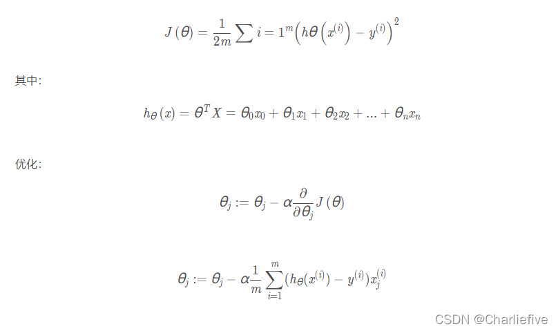
现在让我们使用梯度下降来实现线性回归,以最小化成本函数。 以下代码示例中实现的方程在“练习”文件夹中的“ex1.pdf”中有详细说明。
首先,我们将创建一个以参数θ为特征函数的代价函数
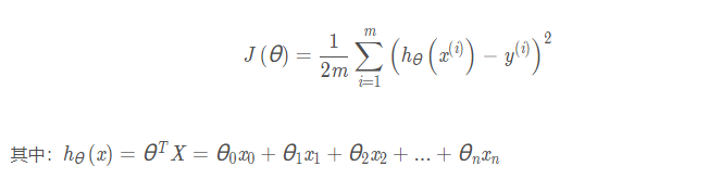 计算代价函数 J ( θ )
'''
作用:计算代价函数,向量化来计算参数
:param X: 输入矩阵
:param y: 输出目标
:param theta: parameters
:return:
'''
def computeCost(X, y, theta):

    inner = np.power(((X * theta.T) - y), 2)
    # print(inner)
    return np.sum(inner) / (2 * len(X))
让我们在训练集中添加一列,以便我们可以使用向量化的解决方案来计算代价和梯度。
data.insert(0, 'Ones', 1)       # 增加一条第一列,全部数值为1
# print(data)
现在我们来做一些变量初始化。
取最后一列为 y,其余为 X
观察下 X (训练集) and y (目标变量)是否正确.
# 变量初始化:set X (training data) and y (target variable)
cols = data.shape[1]  # 列数
X = data.iloc[:, 0:cols - 1]        # 取前cols-1列,即输入向量
y = data.iloc[:, cols - 1:cols]     # 取最后一列作为目标向量
# print(X.head()) # 观察下 X (训练集) and y (目标变量)是否正确.
# print(y.head())
但是matrix的优势就是相对简单的运算符号,比如两个矩阵相乘,就是用符号*,但是array相乘不能这么用,得用方法.dot()
array的优势就是不仅仅表示二维,还能表示3、4、5…维,而且在大部分Python程序里,array也是更常用的。
两者区别:
对应元素相乘:matrix可以用np.multiply(X2,X1),array直接X1X2
点乘:matrix直接X1X2,array可以 X1@X2 或 X1.dot(X2) 或 np.dot(X1, X2)
代价函数是应该是numpy矩阵,所以我们需要转换X和Y,然后才能使用它们。 我们还需要初始化theta。
X = np.matrix(X.values)
y = np.matrix(y.values)
theta = np.matrix([0,0]) # theta 是一个(1,2)矩阵
computeCost(X, y, theta)
# print(X.shape, y.shape, theta.shape)  # 查看各自的行列数
# print(computeCost(X, y, theta)) # 32.072733877455676
batch gradient decent(批量梯度下降)
初始化一些附加变量 - 学习速率α和要执行的迭代次数。并开始计算合适的theta,写出梯度下降算法的函数。
alpha = 0.01 # 学习速率α
epoch = 1000 # 要执行的迭代次数
'''
2.作用:获得最终梯度下降后的theta值以及cost
:param X:
:param y:
:param theta:
:param alpha:
:param epoch:
:return:
'''
def gradientDescent(X, y, theta, alpha, epoch):
# 变量初始化,储存数据
np.matrix(np.zeros(theta.shape)) # 初始化一个临时矩阵(1, 2)
# flatten()降维 即返回一个折叠成一维的数组。但是该函数只能适用于numpy对象,即array或者mat,普通的list列表是不行的。
parameters = int(theta.flatten().shape[1]) # 参数theta的数量 2
# print(parameters)
cost = np.zeros(epoch) # 初始化一个ndarray, 包含每次训练后的cost #1000个0的矩阵
# print(cost)
counterTheta = np.zeros((epoch, 2)) #1000 * 2的数组
m = X.shape[0] # 样本参数 97行
for i in range(epoch):
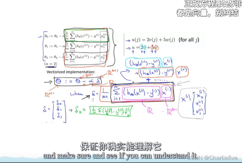
'''
使用 vectorization同时更新所有的θ,可以大大提高效率,此处都是相对应的进行计算
X.shape, theta.shape, y.shape, X.shape[0]
((97, 2), (1, 2), (97, 1), 97)
'''
# 相当于theta1 theta2不停做偏导并且更新 theta[theta1, theta2] temp是临时的theta
temp = theta - (alpha / m) * (X * theta.T - y).T * X
theta = temp
counterTheta[i] = theta
cost[i] = computeCost(X, y, theta)
pass
return counterTheta, theta, cost
调用梯度下降函数
counterTheta, final_theta, cost = gradientDescent(X, y, theta, alpha, epoch)
computeCost(X, y, final_theta)
# print(computeCost(X, y, final_theta)) # 4.515955503078912
画图
x = np.linspace(data.Population.min(), data.Population.max(), 100)  # xlabel start:返回样本数据开始点 stop:返回样本数据结束点 num:生成的样本数据量,默认为50
f = final_theta[0, 0] + (final_theta[0, 1] * x)  # ylabel profit
print(final_theta)


fig1, ax = plt.subplots(figsize=(6, 4)) # 尺寸
ax.plot(x, f, 'r', label='Predictionnnnnn') # 横坐标 纵坐标 颜色 标签
ax.scatter(data.Population, data.Profit, label='Training Data') # 点的离散值
ax.legend(loc=2) # 2表示在左上角
ax.set_xlabel('Population')
ax.set_ylabel('Profit')
ax.set_title('Predicted Profit vs. Population Size')

fig2, ax = plt.subplots(figsize=(8, 4))
ax.plot(np.arange(epoch), cost, 'r') # 横坐标 纵坐标 颜色
ax.set_xlabel('Iteration')
ax.set_ylabel('Cost')
ax.set_title('Error vs. Training Epoch')
plt.show()
完整代码
# Kyrie Irving
# !/9462...
import numpy as np
import pandas as pd
import matplotlib.pyplot as plt

'''
作用:计算代价函数,向量化来计算参数
:param X: 输入矩阵
:param y: 输出目标
:param theta: parameters
:return:
'''
def computeCost(X, y, theta):

    inner = np.power(((X * theta.T) - y), 2)
    # print(inner)
    return np.sum(inner) / (2 * len(X))

'''
2.作用:获得最终梯度下降后的theta值以及cost
:param X:
:param y:
:param theta:
:param alpha:
:param epoch:
:return:
'''
def gradientDescent(X, y, theta, alpha, epoch):
    # 变量初始化,储存数据
    np.matrix(np.zeros(theta.shape)) # 初始化一个临时矩阵(1, 2)
    # flatten()降维 即返回一个折叠成一维的数组。但是该函数只能适用于numpy对象,即array或者mat,普通的list列表是不行的。
    parameters = int(theta.flatten().shape[1]) # 参数theta的数量 2
    # print(parameters)
    cost = np.zeros(epoch)  # 初始化一个ndarray, 包含每次训练后的cost #1000个0的矩阵
    # print(cost)
    counterTheta = np.zeros((epoch, 2)) #1000 * 2的数组
    m = X.shape[0]  # 样本参数 97行

    for i in range(epoch):
        '''
        使用 vectorization同时更新所有的θ,可以大大提高效率,此处都是相对应的进行计算
        X.shape, theta.shape, y.shape, X.shape[0]
        ((97, 2), (1, 2), (97, 1), 97)
        '''
        # 相当于theta1 theta2不停做偏导并且更新 theta[theta1, theta2] temp是临时的theta
        temp = theta - (alpha / m) * (X * theta.T - y).T * X
        theta = temp
        counterTheta[i] = theta
        cost[i] = computeCost(X, y, theta)
        pass
    return counterTheta, theta, cost


'''
单变量线性回归
1.Prepare datasets
'''
path = 'ex1data1.txt'
# names添加列名,header用指定的行来作为标题,若原无标题且指定标题则设为None
data = pd.read_csv(path, header=None, names=['Population', 'Profit'])
data.head()
data.describe()
# print(data.head())#显示前五行
# print(data.describe())

# 展示散点图,可视化理解数据
# data.plot(kind='scatter', x='Population', y='Profit', figsize=(8,5))
# plt.title("Scatter plot of training data") #添加描述信息
# plt.xlabel("population of city")
# plt.ylabel("profit")
# plt.show()

data.insert(0, 'Ones', 1)       # 增加一条第一列,全部数值为1
# print(data)

# 变量初始化:set X (training data) and y (target variable)
cols = data.shape[1]  # 列数
X = data.iloc[:, 0:cols - 1]        # 取前cols-1列,即输入向量
y = data.iloc[:, cols - 1:cols]     # 取最后一列作为目标向量
# print(X.head()) # 观察下 X (训练集) and y (目标变量)是否正确.
# print(y.head())

X = np.matrix(X.values)
y = np.matrix(y.values)
theta = np.matrix([0,0]) # theta 是一个(1,2)矩阵
computeCost(X, y, theta)
# print(X.shape, y.shape, theta.shape)  # 查看各自的行列数
# print(computeCost(X, y, theta)) # 32.072733877455676

alpha = 0.01 # 学习速率α
epoch = 1000 # 要执行的迭代次数
counterTheta, final_theta, cost = gradientDescent(X, y, theta, alpha, epoch)
computeCost(X, y, final_theta)
# print(computeCost(X, y, final_theta)) # 4.515955503078912

x = np.linspace(data.Population.min(), data.Population.max(), 100)  # xlabel start:返回样本数据开始点 stop:返回样本数据结束点 num:生成的样本数据量,默认为50
f = final_theta[0, 0] + (final_theta[0, 1] * x)  # ylabel profit
print(final_theta)


fig1, ax = plt.subplots(figsize=(6, 4)) # 尺寸
ax.plot(x, f, 'r', label='Predictionnnnnn') # 横坐标 纵坐标 颜色 标签
ax.scatter(data.Population, data.Profit, label='Training Data') # 点的离散值
ax.legend(loc=2) # 2表示在左上角
ax.set_xlabel('Population')
ax.set_ylabel('Profit')
ax.set_title('Predicted Profit vs. Population Size')

fig2, ax = plt.subplots(figsize=(8, 4))
ax.plot(np.arange(epoch), cost, 'r') # 横坐标 纵坐标 颜色
ax.set_xlabel('Iteration')
ax.set_ylabel('Cost')
ax.set_title('Error vs. Training Epoch')
plt.show()
多变量线性回归
练习1还包括一个房屋价格数据集,其中有2个变量(房子的大小,卧室的数量)和目标(房子的价格)。 我们使用我们已经应用的技术来分析数据集。
数据
2104,3,399900
1600,3,329900
2400,3,369000
1416,2,232000
3000,4,539900
1985,4,299900
1534,3,314900
1427,3,198999
1380,3,212000
1494,3,242500
1940,4,239999
2000,3,347000
1890,3,329999
4478,5,699900
1268,3,259900
2300,4,449900
1320,2,299900
1236,3,199900
2609,4,499998
3031,4,599000
1767,3,252900
1888,2,255000
1604,3,242900
1962,4,259900
3890,3,573900
1100,3,249900
1458,3,464500
2526,3,469000
2200,3,475000
2637,3,299900
1839,2,349900
1000,1,169900
2040,4,314900
3137,3,579900
1811,4,285900
1437,3,249900
1239,3,229900
2132,4,345000
4215,4,549000
2162,4,287000
1664,2,368500
2238,3,329900
2567,4,314000
1200,3,299000
852,2,179900
1852,4,299900
1203,3,239500
完整代码
# Kyrie Irving
# !/9462...
import numpy as np
import pandas as pd
import matplotlib.pyplot as plt

path = 'ex1data2.txt'
data = pd.read_csv(path, names=['Size', 'Bedrooms', 'Price'])
# 数据归一化后,最优解的寻优过程明显会变得平缓,更容易正确的收敛到最优解。简而言之,归一化的目的就是使得预处理的数据被限定在一定的范围内(比如[0,1]或者[-1,1]),从而消除奇异样本数据导致的不良影响。
data = (data - data.mean()) / data.std() # data2.std()是标准差
data.head()
# print(data.head())
# add ones column
data.insert(0, 'Ones', 1)

# set X (training data) and y (target variable)
cols = data.shape[1]
X = data.iloc[:, 0:cols - 1]
y = data.iloc[:, cols - 1:cols]

# convert to matrices and initialize theta
X = np.matrix(X.values)
y = np.matrix(y.values)
theta = np.matrix(np.array([0, 0, 0])) # 此时theta的维度应该是3

'''
作用:计算代价函数,向量化来计算参数
:param X: 输入矩阵
:param y: 输出目标
:param theta: parameters
:return:
'''
def computeCost(X, y, theta):

    inner = np.power(((X * theta.T) - y), 2)
    # print(inner)
    return np.sum(inner) / (2 * len(X))
# print(computeCost(X, y, theta)) # 0.4893617021276595

'''
2.作用:获得最终梯度下降后的theta值以及cost
:param X:
:param y:
:param theta:
:param alpha:
:param epoch:
:return:
'''
def gradientDescent(X, y, theta, alpha, epoch):
    # 变量初始化,储存数据
    np.matrix(np.zeros(theta.shape)) # 初始化一个临时矩阵(1, 2)
    # flatten()降维 即返回一个折叠成一维的数组。但是该函数只能适用于numpy对象,即array或者mat,普通的list列表是不行的。
    parameters = int(theta.flatten().shape[1]) # 参数theta的数量 2
    # print(parameters)
    cost = np.zeros(epoch)  # 初始化一个ndarray, 包含每次训练后的cost #1000个0的矩阵
    # print(cost)
    counterTheta = np.zeros((epoch, 3)) #1000 * 3的数组
    m = X.shape[0]  # 样本参数 97行

    for i in range(epoch):
        '''
        使用 vectorization同时更新所有的θ,可以大大提高效率,此处都是相对应的进行计算
        X.shape, theta.shape, y.shape, X.shape[0]
        ((97, 2), (1, 2), (97, 1), 97)
        '''
        # 相当于theta1 theta2不停做偏导并且更新 theta[theta1, theta2] temp是临时的theta
        temp = theta - (alpha / m) * (X * theta.T - y).T * X
        theta = temp
        counterTheta[i] = theta
        cost[i] = computeCost(X, y, theta) # 记录每次的cost
        pass
    return counterTheta, theta, cost

'''
3.Run model and Plot
'''
alpha = 0.01
epoch = 3800
counterTheta, final_theta, cost = gradientDescent(X, y, theta, alpha, epoch)
computeCost(X, y, final_theta)
# print(computeCost(X, y, final_theta)) #0.13068648053904253

fig2, ax = plt.subplots(figsize=(8, 4))
ax.plot(np.arange(epoch), cost, 'r')
ax.set_xlabel('Iteration')
ax.set_ylabel('Cost')
ax.set_title('Error vs. Training Epoch')
plt.show()


 1607
1607


 被折叠的 条评论
为什么被折叠?
被折叠的 条评论
为什么被折叠?
 到【灌水乐园】发言


