Python3《机器学习实战》学习笔记（十）：ANN人工神经网络代码详解（数字识别案例以及人脸识别案例）

一、构建基本代码结构

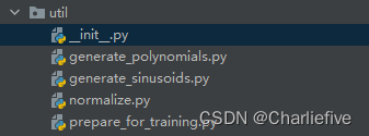
1.1预处理数据的工具包

"""Dataset Features Related Utils"""

from .normalize import normalize
from .generate_polynomials import generate_polynomials
from .generate_sinusoids import generate_sinusoids
from .prepare_for_training import prepare_for_training

"""Add polynomial features to the features set"""

import numpy as np
from .normalize import normalize


def generate_polynomials(dataset, polynomial_degree, normalize_data=False):
    """Extends data set with polynomial features of certain degree.

    Returns a new feature array with more features, comprising of
    x1, x2, x1^2, x2^2, x1*x2, x1*x2^2, etc.

    :param dataset: dataset that we want to generate polynomials for.
    :param polynomial_degree: the max power of new features.
    :param normalize_data: flag that indicates whether polynomials need to normalized or not.
    """

    # Split features on two halves.
    features_split = np.array_split(dataset, 2, axis=1)
    dataset_1 = features_split[0]
    dataset_2 = features_split[1]

    # Extract sets parameters.
    (num_examples_1, num_features_1) = dataset_1.shape
    (num_examples_2, num_features_2) = dataset_2.shape

    # Check if two sets have equal amount of rows.
    if num_examples_1 != num_examples_2:
        raise ValueError('Can not generate polynomials for two sets with different number of rows')

    # Check if at list one set has features.
    if num_features_1 == 0 and num_features_2 == 0:
        raise ValueError('Can not generate polynomials for two sets with no columns')

    # Replace empty set with non-empty one.
    if num_features_1 == 0:
        dataset_1 = dataset_2
    elif num_features_2 == 0:
        dataset_2 = dataset_1

    # Make sure that sets have the same number of features in order to be able to multiply them.
    num_features = num_features_1 if num_features_1 < num_examples_2 else num_features_2
    dataset_1 = dataset_1[:, :num_features]
    dataset_2 = dataset_2[:, :num_features]

    # Create polynomials matrix.
    polynomials = np.empty((num_examples_1, 0))

    # Generate polynomial features of specified degree.
    for i in range(1, polynomial_degree + 1):
        for j in range(i + 1):
            polynomial_feature = (dataset_1 ** (i - j)) * (dataset_2 ** j)
            polynomials = np.concatenate((polynomials, polynomial_feature), axis=1)

    # Normalize polynomials if needed.
    if normalize_data:
        polynomials = normalize(polynomials)[0]

    # Return generated polynomial features.
    return polynomials

"""Add sinusoid features to the features set"""

import numpy as np


def generate_sinusoids(dataset, sinusoid_degree):
    """Extends data set with sinusoid features.

    Returns a new feature array with more features, comprising of
    sin(x).

    :param dataset: data set.
    :param sinusoid_degree: multiplier for sinusoid parameter multiplications
    """

    # Create sinusoids matrix.
    num_examples = dataset.shape[0]
    sinusoids = np.empty((num_examples, 0))

    # Generate sinusoid features of specified degree.
    for degree in range(1, sinusoid_degree + 1):
        sinusoid_features = np.sin(degree * dataset)
        sinusoids = np.concatenate((sinusoids, sinusoid_features), axis=1)

    # Return generated sinusoidal features.
    return sinusoids

"""Normalize features"""

import numpy as np


def normalize(features):
    """Normalize features.

    Normalizes input features X. Returns a normalized version of X where the mean value of
    each feature is 0 and deviation is close to 1.

    :param features: set of features.
    :return: normalized set of features.
    """

    # Copy original array to prevent it from changes.
    features_normalized = np.copy(features).astype(float)

    # Get average values for each feature (column) in X.
    features_mean = np.mean(features, 0)

    # Calculate the standard deviation for each feature.
    features_deviation = np.std(features, 0)

    # Subtract mean values from each feature (column) of every example (row)
    # to make all features be spread around zero.
    if features.shape[0] > 1:
        features_normalized -= features_mean

    # Normalize each feature values so that all features are close to [-1:1] boundaries.
    # Also prevent division by zero error.
    features_deviation[features_deviation == 0] = 1
    features_normalized /= features_deviation

    return features_normalized, features_mean, features_deviation

"""Prepares the dataset for training"""

import numpy as np
from .normalize import normalize
from .generate_sinusoids import generate_sinusoids
from .generate_polynomials import generate_polynomials


def prepare_for_training(data, polynomial_degree=0, sinusoid_degree=0, normalize_data=True):
    """Prepares data set for training on prediction"""

    # Calculate the number of examples.
    num_examples = data.shape[0]

    # Prevent original data from being modified.
    data_processed = np.copy(data)

    # Normalize data set.
    features_mean = 0
    features_deviation = 0
    data_normalized = data_processed
    if normalize_data:
        (
            data_normalized,
            features_mean,
            features_deviation
        ) = normalize(data_processed)

        # Replace processed data with normalized processed data.
        # We need to have normalized data below while we will adding polynomials and sinusoids.
        data_processed = data_normalized

    # Add sinusoidal features to the dataset.
    if sinusoid_degree > 0:
        sinusoids = generate_sinusoids(data_normalized, sinusoid_degree)
        data_processed = np.concatenate((data_processed, sinusoids), axis=1)

    # Add polynomial features to data set.
    if polynomial_degree > 0:
        polynomials = generate_polynomials(data_normalized, polynomial_degree, normalize_data)
        data_processed = np.concatenate((data_processed, polynomials), axis=1)

    # Add a column of ones to X.
    data_processed = np.hstack((np.ones((num_examples, 1)), data_processed))

    return data_processed, features_mean, features_deviation

1.2 初始化参数

    def __init__(self, data, labels, layers, normalize_data=False):
        data_processed = prepare_for_training(data, normalize_data = normalize_data)[0]
        self.data = data_processed
        self.labels = labels
        self.layers = layers    # 28*28*1=784 25（隐层可以改） 10(最后输出结果)
        self.normalize_data = normalize_data
        self.thetas = MultilayerPerceptron.thetas_init(layers)

1.3工具类sigmoid

    @staticmethod
    def sigmoid(z):
        """Sigmoid 函数"""
        return 1.0 / (1.0 + np.exp(-np.asarray(z)))

    @staticmethod
    def sigmoid_gradient(z):
        """计算Sigmoid 函数的梯度"""
        g = np.zeros_like(z)
        # ======================　你的代码 ======================

        # 计算Sigmoid 函数的梯度g的值
        dz = MultilayerPerceptron.sigmoid(z)
        g = dz * (1 - dz)
        # =======================================================
        return g

1.4工具类矩阵变换

    '''
    将矩阵拉长变成1*n
    '''
    @staticmethod
    def thetas_unroll(thetas):
        num_thetas = len(thetas)
        unrolled_theta = np.array([])
        for num_thetas_index in range(num_thetas):
            unrolled_theta = np.hstack((unrolled_theta, thetas[num_thetas_index].flatten()))
        return unrolled_theta

    '''
    将1*n变成矩阵
    '''
    @staticmethod
    def thetas_roll(unrolled_thetas, layers):
        num_layers = len(layers)
        thetas = {}
        unrolled_shift = 0
        for index in range(num_layers - 1):
            in_count = int(layers[index])
            out_count = int(layers[index+1])

            theta_width = in_count + 1
            theta_height = out_count
            theta_volume = theta_width * theta_height
            start_index = unrolled_shift
            end_index = unrolled_shift + theta_volume

            layer_theta_unrolled = unrolled_thetas[start_index: end_index]
            thetas[index] = layer_theta_unrolled.reshape((theta_height, theta_width))
            unrolled_shift += theta_volume
        return thetas

1.5初始化theta

    '''
    初始化theta
    '''
    @staticmethod
    def thetas_init(layers):
        num_layers = len(layers)
        thetas = {}
        for layer_index in range(num_layers - 1):
            '''
            执行两次，得到两组参数矩阵：25*785 10*26
            '''
            in_count = int(layers[layer_index])
            out_count = int(layers[layer_index + 1])
            # print(type(in_count))
            # 这里考虑偏置项，偏置的个数和输出的结果是一致的
            randomTheta = np.random.rand(out_count, in_count + 1) * 0.05  # 随机初始化 值尽量小点
            # print(randomTheta)
            thetas[layer_index] = randomTheta

            print(thetas[layer_index].shape)
        return thetas

1.6正向传播

'''
    计算损失函数
    '''
    @staticmethod
    def cost_function(data, labels, thetas, layers):
        num_layers = len(layers)
        num_examples = data.shape[0]
        num_labels = layers[-1]

        # 正向传播
        predictions = MultilayerPerceptron.feedforward_propagation(data, thetas, layers)
        # 制作标签，每个样本对应的都是one-hot
        bitwise_labels = np.zeros((num_examples, num_labels))
        for example_index in range(num_examples):
            bitwise_labels[example_index][labels[example_index][0]] = 1
        # 这里有很大很大的疑问
        bit_set_cost = np.sum(np.log(predictions[bitwise_labels == 1])) # 预测正确的
        bit_not_set_cost = np.sum(np.log(1 - predictions[bitwise_labels == 1])) # 我感觉自己是正确的
        cost = (-1 / num_examples) * (bit_set_cost + bit_not_set_cost)
        return cost
    '''
    正向传播
    '''
    @staticmethod
    def feedforward_propagation(data, thetas, layers):
        num_layers = len(layers)
        num_examples = data.shape[0]
        in_layer_activation = data

        for index in range(num_layers - 1):
            theta = thetas[index]
            print(theta.shape)
            out_layer_activation = MultilayerPerceptron.sigmoid(np.dot(in_layer_activation, theta.T))   # 1700*785  785*25
            # 正常计算完是num_examples * 25 需要多加一列 变成num_examples * 26
            out_layer_activation = np.hstack((np.ones((num_examples, 1)), out_layer_activation))
            in_layer_activation = out_layer_activation

        # 去除偏置项
        return in_layer_activation[:, 1:]

1.7反向传播

    '''
    反向传播
    '''
    @staticmethod
    def back_propagation(data, labels, thetas, layers):
        num_layers = len(layers)
        num_examples = data.shape[0]
        num_features = data.shape[1]
        num_label_types = layers[-1]

        deltas = {}

        # 初始化操作
        for index in range(num_layers - 1):
            in_count = layers[index]
            out_count = layers[index + 1]
            # 这一步很难理解，但是实际上生成的是三层神经网络中间产生两次的中间矩阵
            # 第一个是 25 * 785 第二个是 10 * 26
            deltas[index] = np.zeros((out_count, in_count + 1))

        for example_index in range(num_examples):
            layer_inputs = {}
            layer_activations = {}
            layer_activation = data[example_index, :].reshape((num_features, 1))    # 785*1    初始元素
            layer_activations[0] = layer_activation
            # 逐层计算
            for index in range(num_layers - 1):
                layer_theta = thetas[index]  # 25*785 10*26
                # 与前向传播不同的是 这里与theta相乘的不是完整数据集 而是每个样本单独转置后的结果 785*1
                layer_input = MultilayerPerceptron.sigmoid(np.dot(layer_theta, layer_activation))
                layer_activation = np.vstack((np.array([[1]]), layer_input))
                layer_inputs[index + 1] = layer_input   # 后一层计算结果
                layer_activations[index + 1] = layer_activation # 后一层经过多加了一列的结果
            # !!!!!!!!!!!!
            output_layer_activation = layer_activation[1:, :]

            delta = {}
            # 标签处理
            bitwise_label = np.zeros((num_label_types, 1))
            bitwise_label[labels[example_index][0]] = 1

            # 计算输出层和真实值之间的差异
            delta[num_layers - 1] = output_layer_activation - bitwise_label # 10*1
            # 循环遍历 L L-1 L-2...2 这里直接套视频里的公式即可
            for index in range(num_layers - 2, 0, -1):
                layer_theta = thetas[index]
                next_delta = delta[index + 1]
                layer_input = layer_inputs[index]
                layer_input = np.vstack((np.array([[1]]), layer_input))
                # 按照公式推
                delta[index] = np.dot(layer_theta.T, next_delta) * MultilayerPerceptron.sigmoid_gradient(layer_input)
                # 过滤掉偏置参数
                delta[index] = delta[index][1:, :]
            for index in range(num_layers - 1):
                layer_delta = np.dot(delta[index+1], layer_activations[index].T)
                # 第一次是 25*785 第二次是10*26
                deltas[index] = deltas[index] + layer_delta

        for index in range(num_layers - 1):
            deltas[index] /= num_examples

        return deltas

1.8梯度下降

    '''
    梯度..
    '''
    @staticmethod
    def gradient_step(data, labels, optimized_theta, layers):
        theta = MultilayerPerceptron.thetas_roll(optimized_theta, layers)
        thetas_rolled_gradients = MultilayerPerceptron.back_propagation(data, labels, theta, layers)
        thetas_unrolled_gradients = MultilayerPerceptron.thetas_unroll(thetas_rolled_gradients)
        return thetas_unrolled_gradients



    '''
    梯度下降算法
    '''
    @staticmethod
    def gradient_descent(data, labels, unrolled_theta, layers, max_iter, alpha):
        optimized_theta = unrolled_theta    # 最终theta结果
        cost_history = []
        for index in range(max_iter):
            # 这里记得要及时更新theta
            cost = MultilayerPerceptron.cost_function(data, labels, MultilayerPerceptron.thetas_roll(optimized_theta, layers), layers)
            # cost = MultilayerPerceptron.cost_function(data, labels, MultilayerPerceptron.thetas_roll(unrolled_theta, layers), layers)
            cost_history.append(cost)
            # 得到最终梯度结果 进行参数更新操作
            theta_gradient = MultilayerPerceptron.gradient_step(data, labels, optimized_theta, layers)
            # 更新操作
            optimized_theta -= alpha * theta_gradient
        return optimized_theta, cost_history

1.9训练模块

    '''
    训练模块
    '''
    def train(self, max_iter = 1000, alpha = 0.1):
        unrolled_theta = MultilayerPerceptron.thetas_unroll(self.thetas)

        optimized_theta, cost_history = MultilayerPerceptron.gradient_descent(self.data, self.labels, unrolled_theta, self.layers, max_iter, alpha)

        self.thetas = MultilayerPerceptron.thetas_roll(optimized_theta, self.layers)

        return self.thetas, cost_history

二、MNIST数字识别

MNIST是知名数字数据集，大家可以百度搜索资源，这里使用的是csv文件进行识别。

import numpy as np
import pandas as pd
import matplotlib.pyplot as plt
import matplotlib.image as mping
import math

from ANN.MultilayerPerceptron import MultilayerPerceptron

data = pd.read_csv('data/mnist_csv/mnist_train.csv')
data2 = pd.read_csv('data/mnist_csv/mnist_test.csv')
# numbers_to_display = 25 # 一次展示25个图
# num_cell = math.ceil(math.sqrt(numbers_to_display))
# plt.figure(figsize=(10, 10))
# for index in range(numbers_to_display):
#     digit = data[index: index+1].values
#     # print(digit.shape)
#     digit_label = digit[0][0]
#     digit_pixels = digit[0][1:]
#     img_size = int(math.sqrt(digit_pixels.shape[0]))
#     frame = digit_pixels.reshape((img_size, img_size))  # 点点转为矩阵
#     plt.subplot(num_cell, num_cell, index + 1)
#     plt.imshow(frame, cmap='Greys')
#     plt.title(digit_label)
# plt.subplots_adjust(wspace=0.5, hspace=0.5) # 调整每个子图外边距
# plt.show()

train_data = data.sample(frac=0.1)
test_data = data2.sample(frac=0.1)
train_data = train_data.values
test_data = test_data.values

x_train = train_data[:, 1:]
y_train = train_data[:, [0]]
x_test = test_data[:, 1:]
y_test = test_data[:, [0]]

layers = [784, 25, 10]

normalize_data = True
max_iter = 300
alpha = 0.1

multilayer_perceptron = MultilayerPerceptron(x_train, y_train, layers, normalize_data)
thetas, costs = multilayer_perceptron.train(max_iter, alpha)
plt.plot(range(len(costs)), costs)
plt.xlabel('梯度下降step')
plt.ylabel('cost')
plt.show()

y_train_predictions = multilayer_perceptron.predict(x_train)
y_test_predictions = multilayer_perceptron.predict(x_test)

train_p = np.sum(y_train_predictions == y_train)/y_train.shape[0] * 100
test_p = np.sum(y_test_predictions == y_test)/y_test.shape[0] * 100
print("训练准确率：", train_p)
print("测试准确率：", test_p)


训练准确率： 73.8
测试准确率： 74.2

三、人脸识别

数据集在课本上给出的网站上，但是我们先对数据进行处理，将图片转化为合适的像素矩阵，标签也要转化为适合处理的矩阵。

import numpy as np
import os
from PIL import Image
import matplotlib.pyplot as plt
from ANN.MultilayerPerceptron import MultilayerPerceptron


def imgval(example):#定义将图片转化为矩阵的方法
    values=[]
    for i in range(0,example.width):#循环图片的每一行
        for j in range(0,example.height):#循环图片的每一列
            values.append(example.getpixel((i,j))/100)#对图片的rgb值进行缩小处理
    # values=np.array(values)#返回成numpy数组形式
    return values


'''
定义读取图片的方法
'''
def readimg(path):
    returndict = {}
    # os.walk是通过深度优先遍历 home是每次遍历的文件夹 files是读取每个子文件夹的文件
    for home, dirs, files in os.walk(path): # 读取该文件夹下所有的子文件夹
        for filename in files:  # 读取各个子文件夹下的图片
            val=[]
            im=Image.open(os.path.join(home, filename)) # 定义该图片路径
            val.append(im)
            namelist=filename.split("_")
            if namelist[1]=="left":#给图片打上目标值标签
                val.append([0])
            elif namelist[1]=="right":
                val.append([1])
            elif namelist[1]=="up":
                val.append([2])
            elif namelist[1]=="straight":
                val.append([3])
            # 我们这里把图片和标签拼接
            returndict[filename]=val
    return returndict#返回图片字典

'''
把所有图片转化为矩阵 标签转化为列表
'''
def picTwoXY(Imgs):
    x_train = []
    y_train = []
    for img in Imgs:
        x_train.append(imgval(img[0]))
        y_train.append(img[-1])
    return x_train, y_train

trainimgsrc='data/faces'    # 定义训练集文件夹
testimgsrc='data/test'  # 定义测试集文件夹
trainImgs = readimg(trainimgsrc)
testImgs = readimg(testimgsrc)
x_train, y_train = picTwoXY(trainImgs.values())
x_test, y_test = picTwoXY(testImgs.values())
x_train = np.array(x_train)
y_train = np.array(y_train)
x_test = np.array(x_test)
y_test = np.array(y_test)
print(type(x_train))
print(type(y_train))
print(x_train.shape)

layers = [960, 25, 4]

normalize_data = True
max_iter = 300
alpha = 0.1

multilayer_perceptron = MultilayerPerceptron(x_train, y_train, layers, normalize_data)
thetas, costs = multilayer_perceptron.train(max_iter, alpha)

plt.plot(range(len(costs)), costs)
plt.xlabel('梯度下降step')
plt.ylabel('cost')
plt.show()

y_train_predictions = multilayer_perceptron.predict(x_train)
y_test_predictions = multilayer_perceptron.predict(x_test)

train_p = np.sum(y_train_predictions == y_train)/y_train.shape[0] * 100
test_p = np.sum(y_test_predictions == y_test)/y_test.shape[0] * 100
print("训练准确率：", train_p)
print("测试准确率：", test_p)

四、总结

学习了ANN，手动实现正反向传播，但是准确率很差，浮动在70-80之间。手动实现的感觉就这水平了，没有pytorch框架运行的准确率高。

希望继续加油2022快点过去吧。