泰坦尼克号幸存者预测

且听风吟hjc

已于 2023-11-01 22:10:26 修改

阅读量658

点赞数

分类专栏：机器学习文章标签：人工智能 python 机器学习 pytorch

于 2023-10-14 21:23:37 首次发布

本文链接：https://blog.csdn.net/weixin_43902823/article/details/133823908

版权

机器学习专栏收录该内容

4 篇文章 0 订阅

订阅专栏

一、数据处理

首先合并数据集，方便同时对两个数据进行清洗

full = train.append(test, ignore_index= True) # 使用append进行纵向堆叠
full.info()

通过info()查看表格内容

RangeIndex: 1309 entries, 0 to 1308
Data columns (total 12 columns):
 #   Column       Non-Null Count  Dtype  
---  ------       --------------  -----  
 0   PassengerId  1309 non-null   int64  
 1   Survived     891 non-null    float64
 2   Pclass       1309 non-null   int64  
 3   Name         1309 non-null   object 
 4   Sex          1309 non-null   object 
 5   Age          1046 non-null   float64
 6   SibSp        1309 non-null   int64  
 7   Parch        1309 non-null   int64  
 8   Ticket       1309 non-null   object 
 9   Fare         1308 non-null   float64
 10  Cabin        295 non-null    object 
 11  Embarked     1307 non-null   object 
dtypes: float64(3), int64(4), object(5)

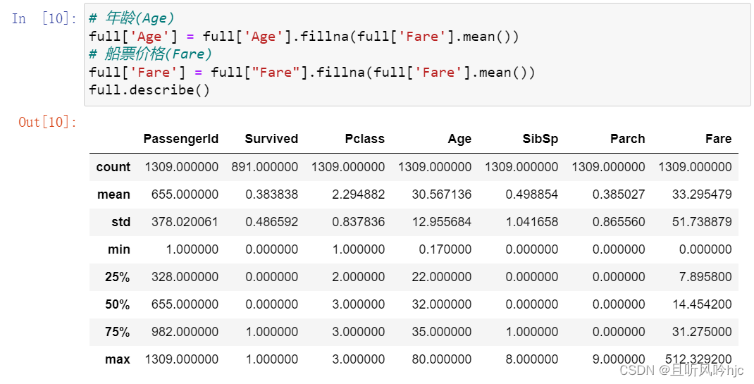
发现Age（年龄）、Fare（票价）、Cabin（船舱号）、Embarked（上船地点）存在缺失，需要进行补充。Name、Sex、Cabin、Embarked数据类型为object，需要进行处理。Ticket为乘客购买的船票编号，默认与存活率无关。

小孩和老人有可能被优先营救，所以年龄是比较关键的数据，必须填充。票价能反映出一个人的经济实力，与存活率相关，也需要进行填充。根据其数据类型，进行平均值填充。

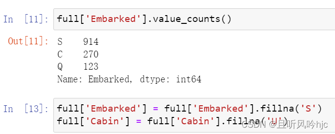
对于登船港口（Embarked），分别计算出各个类别的数量，采用最常见的类别进行填充。对于船舱号（Cabin），由于缺失的数据太多，将缺失的数据用’U’代替，表示未知.

二、特征处理

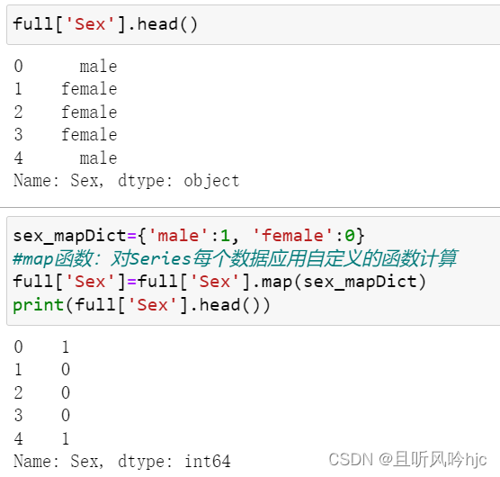
对性别进行处理，男性用1代替，女性用0代替

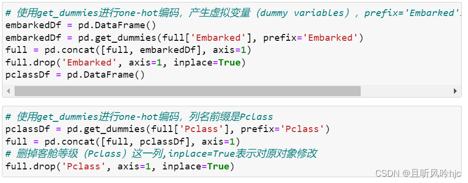
对直接类别的字符串类型使用get_dummies进行one-hot编码，产生虚拟变量（dummy variables）

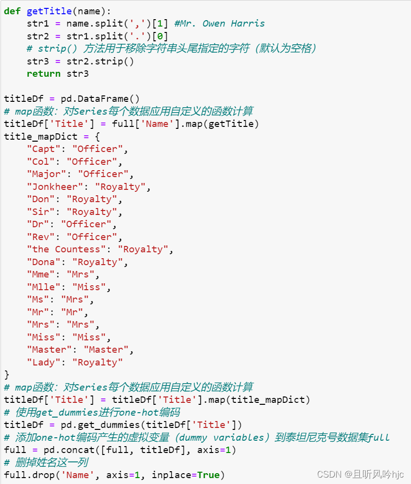
我们可以从名字中可以提取出一个人的头衔，不同的头衔对应不同的社会地位。

Officer政府官员
Royalty王室（皇室）
Mr已婚男士
Mrs已婚妇女
Miss年轻未婚女子
Master有技能的人/教师

通过定义函数getTitle()获取名字头衔，然后根据不同的头衔匹配不同的社会地位。

对于客舱号（Cabin）的处理（与Name 类似），从客舱号中提取客舱类别并进行 one-hot 编码。

对于家庭成员人数与个人生存率也存在着关系，也需要进行处理。

家庭人数=同代直系亲属数（Parch）+不同代直系亲属数（SibSp）+乘客自己

同时我们要根据家庭人数建立家庭类别：
家庭人数=同代直系亲属数（Parch）+不同代直系亲属数（SibSp）+乘客自己
家庭类别：小家庭Family_Single：家庭人数=1；
中等家庭Family_Small: 2<=家庭人数<=4
大家庭Family_Large: 家庭人数>=5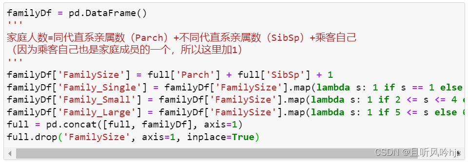

最终处理结果如下表：

PassengerId	Survived	Sex	Age	SibSp	Parch	Fare	Embarked_C	Embarked_Q	Cabin_C	Cabin_D	Family_Single	Family_Small	Family_Large
0	1	0.0	1	22.0	1	A/5 21171	7.2500	0	...	0	1	0	1
1	2	1.0	0	38.0	1	PC 17599	71.2833	1	...	1	0	0	1
2	3	1.0	0	26.0	0	STON/O2. 3101282	7.9250	0	...	0	1	1	0
3	4	1.0	0	35.0	1	113803	53.1000	0	...	1	0	0	1
4	5	0.0	1	35.0	0	373450	8.0500	0	...	0	1	1	0

三、特征选择

通过corr()进行特征选取，构造相关矩阵研究变量之间的相关关系，然后再提取特征，对矩阵中 Survived 那一列输出。

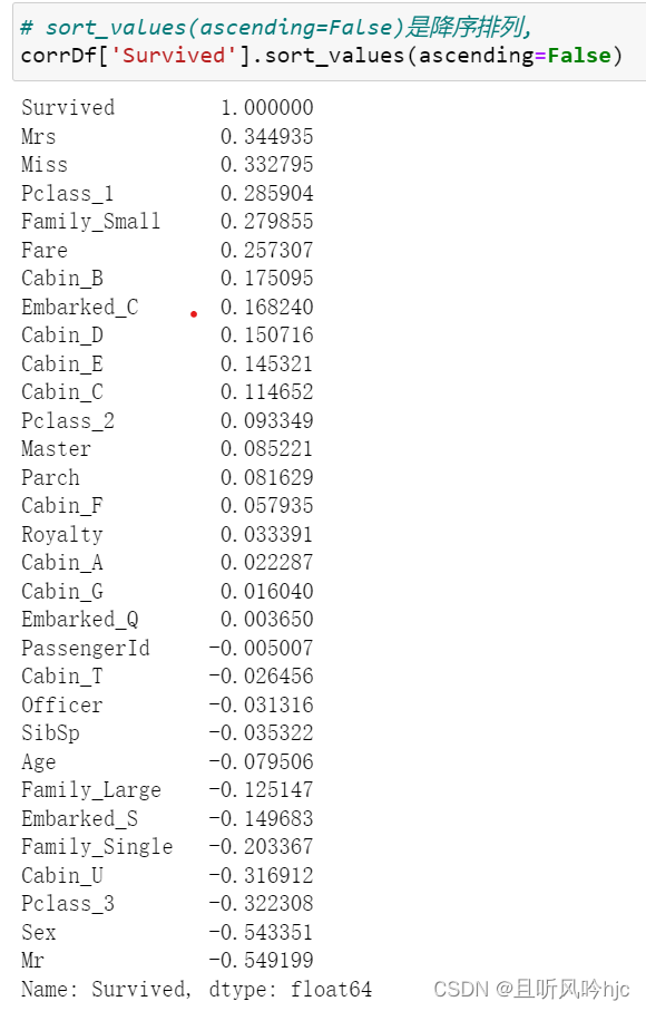
从上图相关性分析中进行选取特征，舍弃负相关的特征，会发现

titleDf,#头衔
pclassDf,#客舱等级
familyDf,#家庭大小
full['Fare'],#船票价格
full['Sex'],#性别
cabinDf,#船舱号
embarkedDf,#登船港口

与存活率有很大的关系，通过pd.concat()函数对这些特征进行拼接。

四、构建模型

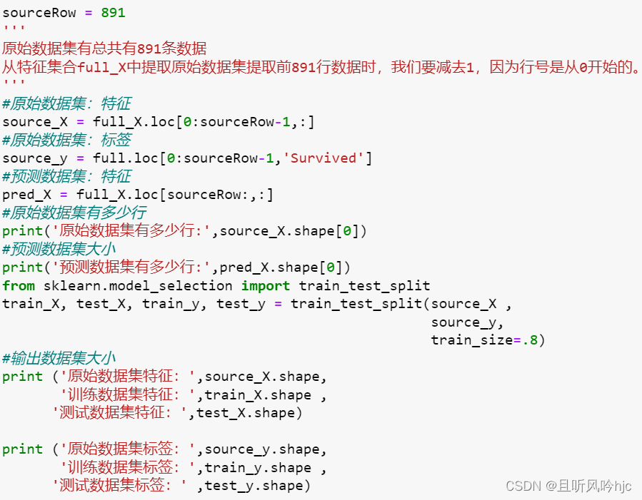
建立训练数据集和测试数据集，从原始数据集（前 891 行数据）中拆分出训练数据集和测试数据集。

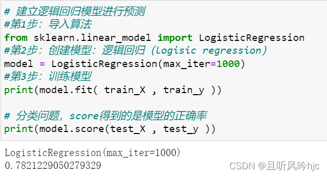
用逻辑回归模型进行预测

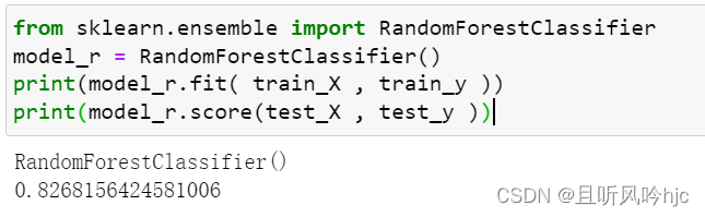
用随机森林模型进行预测

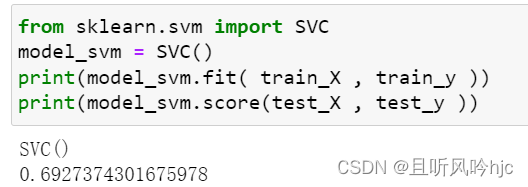
用支持向量机模型进行预测

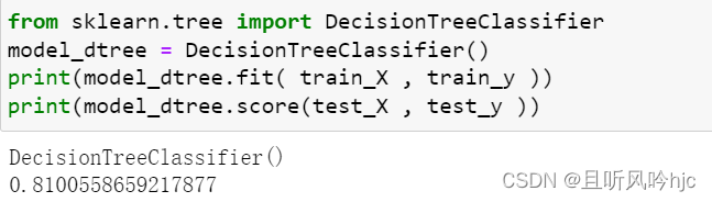
用决策树进行预测

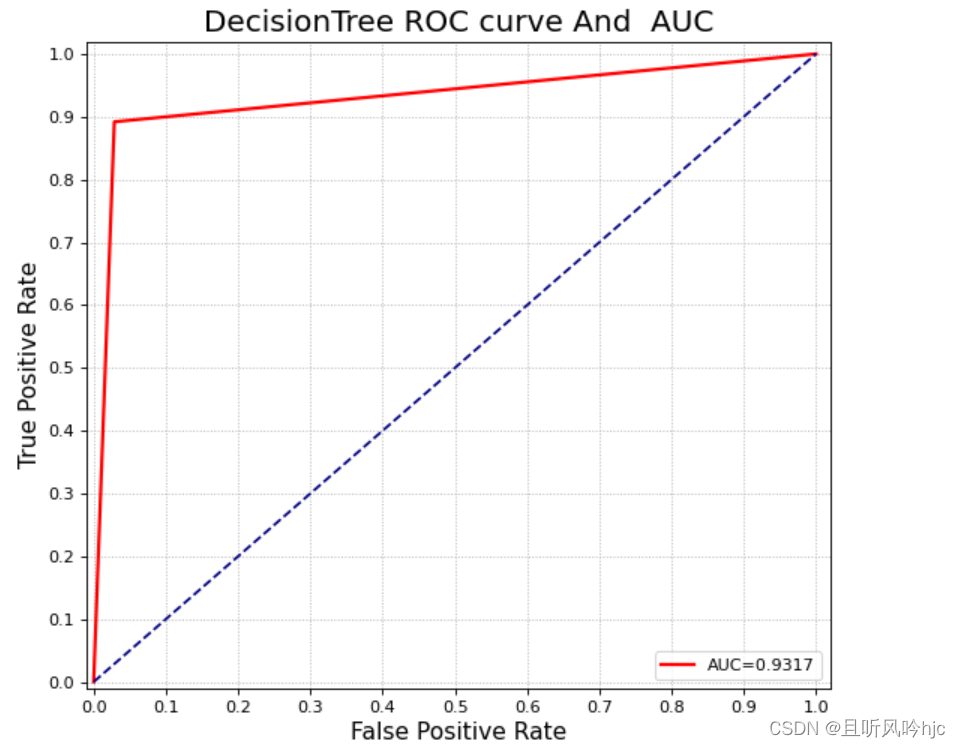
经过比较发现，随机森林的分数较高，对随机森林模型绘制ROC曲线

五、保存结果

用预测数据集到底预测结果，并保存到 csv 文件中

完整代码如下：

# 导入处理数据的包
import numpy as np
import pandas as pd
import matplotlib.pyplot as plt

# 导入数据
# 训练集数据
train = pd.read_csv("data/titanic/train.csv")
# 测试数据集
test = pd.read_csv("data/titanic/test.csv")
print('训练数据集：', train.shape,'测试数据集：', test.shape)
rowNum_train = train.shape[0]
rowNum_test = test.shape[0]
print('Kaggle训练数据集有多少行数据：', rowNum_train,
      'Kaggle测试数据集有多少行数据：', rowNum_test)

# 合并数据集，方便同时对两个数据进行清洗
full = train.append(test, ignore_index= True) # 使用append进行纵向堆叠

# 年龄(Age)
full['Age'] = full['Age'].fillna(full['Fare'].mean())
# 船票价格(Fare)
full['Fare'] = full["Fare"].fillna(full['Fare'].mean())

full['Embarked'] = full['Embarked'].fillna('S')
full['Cabin'] = full['Cabin'].fillna('U')

sex_mapDict={'male':1, 'female':0}
#map函数：对Series每个数据应用自定义的函数计算
full['Sex']=full['Sex'].map(sex_mapDict)

# 使用get_dummies进行one-hot编码，产生虚拟变量（dummy variables），prefix='Embarked'表示列名前缀是Embarked
embarkedDf = pd.DataFrame()
embarkedDf = pd.get_dummies(full['Embarked'], prefix='Embarked')
full = pd.concat([full, embarkedDf], axis=1)
full.drop('Embarked', axis=1, inplace=True)
pclassDf = pd.DataFrame()

# 使用get_dummies进行one-hot编码，列名前缀是Pclass
pclassDf = pd.get_dummies(full['Pclass'], prefix='Pclass')
full = pd.concat([full, pclassDf], axis=1)
# 删掉客舱等级（Pclass）这一列,inplace=True表示对原对象修改
full.drop('Pclass', axis=1, inplace=True)

def getTitle(name):
    str1 = name.split(',')[1] #Mr. Owen Harris
    str2 = str1.split('.')[0]
    # strip() 方法用于移除字符串头尾指定的字符（默认为空格）
    str3 = str2.strip()
    return str3

titleDf = pd.DataFrame()
# map函数：对Series每个数据应用自定义的函数计算
titleDf['Title'] = full['Name'].map(getTitle)
title_mapDict = {
    "Capt": "Officer",
    "Col": "Officer",
    "Major": "Officer",
    "Jonkheer": "Royalty",
    "Don": "Royalty",
    "Sir": "Royalty",
    "Dr": "Officer",
    "Rev": "Officer",
    "the Countess": "Royalty",
    "Dona": "Royalty",
    "Mme": "Mrs",
    "Mlle": "Miss",
    "Ms": "Mrs",
    "Mr": "Mr",
    "Mrs": "Mrs",
    "Miss": "Miss",
    "Master": "Master",
    "Lady": "Royalty"
}
# map函数：对Series每个数据应用自定义的函数计算
titleDf['Title'] = titleDf['Title'].map(title_mapDict)
# 使用get_dummies进行one-hot编码
titleDf = pd.get_dummies(titleDf['Title'])
# 添加one-hot编码产生的虚拟变量（dummy variables）到泰坦尼克号数据集full
full = pd.concat([full, titleDf], axis=1)
# 删掉姓名这一列
full.drop('Name', axis=1, inplace=True)


#存放客舱号信息
cabinDf = pd.DataFrame()

'''
客场号的类别值是首字母，例如：
C85 类别映射为首字母C
'''
full['Cabin'] = full['Cabin'].map(lambda c: c[0])
# lambda c: c[0]客舱号的首字母，U代表不知道属于哪个船舱
# 使用get_dummies进行one-hot编码，列名前缀是Cabin
cabinDf = pd.get_dummies( full['Cabin'] , prefix='Cabin')
full = pd.concat([full, cabinDf], axis=1)

# 删掉客舱号这一列
full.drop('Cabin', axis=1, inplace=True)

familyDf = pd.DataFrame()
'''
家庭人数=同代直系亲属数（Parch）+不同代直系亲属数（SibSp）+乘客自己
（因为乘客自己也是家庭成员的一个，所以这里加1）
'''
familyDf['FamilySize'] = full['Parch'] + full['SibSp'] + 1
familyDf['Family_Single'] = familyDf['FamilySize'].map(lambda s: 1 if s == 1 else 0)
familyDf['Family_Small'] = familyDf['FamilySize'].map(lambda s: 1 if 2 <= s <= 4 else 0)
familyDf['Family_Large'] = familyDf['FamilySize'].map(lambda s: 1 if 5 <= s else 0)
full = pd.concat([full, familyDf], axis=1)
full.drop('FamilySize', axis=1, inplace=True)

# 进行特征选取
# corr()构造相关矩阵研究变量之间的相关关系
corrDf = full.corr()
# sort_values(ascending=False)是降序排列,
corrDf['Survived'].sort_values(ascending=False)
#  头衔#客舱等级#家庭大小#船票价格#性别#船舱号#登船港口
full_X = pd.concat([titleDf, pclassDf, full['Fare'], full['Sex'], cabinDf, embarkedDf], axis=1)

sourceRow = 891
'''
原始数据集有总共有891条数据
从特征集合full_X中提取原始数据集提取前891行数据时，我们要减去1，因为行号是从0开始的。
'''
#原始数据集：特征
source_X = full_X.loc[0:sourceRow-1,:]
#原始数据集：标签
source_y = full.loc[0:sourceRow-1,'Survived']
#预测数据集：特征
pred_X = full_X.loc[sourceRow:,:]
#原始数据集有多少行
print('原始数据集有多少行:',source_X.shape[0])
#预测数据集大小
print('预测数据集有多少行:',pred_X.shape[0])
from sklearn.model_selection import train_test_split
train_X, test_X, train_y, test_y = train_test_split(source_X ,
                                                    source_y,
                                                    train_size=.8)
#输出数据集大小
print ('原始数据集特征：',source_X.shape,
       '训练数据集特征：',train_X.shape ,
      '测试数据集特征：',test_X.shape)

print ('原始数据集标签：',source_y.shape,
       '训练数据集标签：',train_y.shape ,
      '测试数据集标签：' ,test_y.shape)


# 建立逻辑回归模型进行预测
#第1步：导入算法
from sklearn.linear_model import LogisticRegression
#第2步：创建模型：逻辑回归（logisic regression）
model = LogisticRegression(max_iter=1000)
#第3步：训练模型
print(model.fit( train_X , train_y ))

# 分类问题，score得到的是模型的正确率
print(model.score(test_X , test_y ))

from sklearn.ensemble import RandomForestClassifier 
model_r = RandomForestClassifier()
print(model_r.fit( train_X , train_y ))
print(model_r.score(test_X , test_y ))

from sklearn.svm import SVC 
model_svm = SVC()
print(model_svm.fit( train_X , train_y ))
print(model_svm.score(test_X , test_y ))

from sklearn.tree import DecisionTreeClassifier 
model_dtree = DecisionTreeClassifier()
print(model_dtree.fit( train_X , train_y ))
print(model_dtree.score(test_X , test_y ))

y_p = model_r.predict(test_X)
from sklearn.metrics import roc_curve
# 计算 TPR 和 FPR
fpr, tpr, thresholds = roc_curve(test_y, y_p)
# 计算auc
from sklearn.metrics import roc_auc_score
auc = roc_auc_score(test_y, y_p)
# 绘制 ROC 曲线
plt.figure(figsize=(8, 7), dpi=80, facecolor='w')    # dpi:每英寸长度的像素点数；facecolor 背景颜色
plt.xlim((-0.01, 1.02))  # x,y 轴刻度的范围
plt.ylim((-0.01, 1.02))
plt.xticks(np.arange(0, 1.1, 0.1))  #绘制刻度
plt.yticks(np.arange(0, 1.1, 0.1))
plt.plot(fpr, tpr, 'r-', lw=2, label='AUC=%.4f' % auc)  # 绘制AUC 曲线
plt.plot([0, 1], [0, 1], color='navy', linestyle='--')
plt.legend(loc='lower right')    # 设置显示标签的位置
plt.xlabel('False Positive Rate', fontsize=14)   #绘制x,y 坐标轴对应的标签
plt.ylabel('True Positive Rate', fontsize=14)
plt.grid(visible=True, ls=':')  # 绘制网格作为底板;b是否显示网格线；ls表示line style
plt.title(u'DecisionTree ROC curve And  AUC', fontsize=18)  # 打印标题
plt.show()

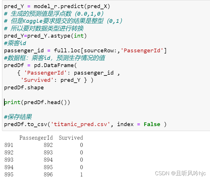
pred_Y = model_r.predict(pred_X)
# 生成的预测值是浮点数（0.0,1,0）
# 但是Kaggle要求提交的结果是整型（0,1）
# 所以要对数据类型进行转换
pred_Y=pred_Y.astype(int)
#乘客id
passenger_id = full.loc[sourceRow:,'PassengerId']
#数据框：乘客id，预测生存情况的值
predDf = pd.DataFrame(
    { 'PassengerId': passenger_id ,
     'Survived': pred_Y } )
predDf.shape

print(predDf.head())

#保存结果
predDf.to_csv('titanic_pred.csv', index = False )

且听风吟hjc

关注

0
点赞
踩
11

收藏

觉得还不错? 一键收藏
1
评论
泰坦尼克号幸存者预测

发现Age（年龄）、Fare（票价）、Cabin（船舱号）、Embarked（上船地点）存在缺失，需要进行补充。对于登船港口（Embarked），分别计算出各个类别的数量，采用最常见的类别进行填充。对于船舱号（Cabin），由于缺失的数据太多，将缺失的数据用’U’代替，表示未知.通过corr()进行特征选取，构造相关矩阵研究变量之间的相关关系，然后再提取特征，对矩阵中 Survived 那一列输出。对于客舱号（Cabin）的处理（与Name 类似），从客舱号中提取客舱类别并进行 one-hot 编码。
复制链接

扫一扫