gee学习笔记第三天

最新推荐文章于 2024-05-23 14:26:49 发布

fix you

最新推荐文章于 2024-05-23 14:26:49 发布

阅读量587

点赞数

分类专栏： gee学习笔记文章标签：学习前端 javascript

本文链接：https://blog.csdn.net/weixin_43908798/article/details/126142768

版权

gee学习笔记专栏收录该内容

3 篇文章 0 订阅

订阅专栏

gee学习笔记第三天

文章目录

gee学习笔记第三天
前言
一、Geometry和Feature
二、Getting image metadata
三、Using the plotting tool和可视化
总结

前言

主要的内容如下
在这里插入图片描述

提示：以下是本篇文章正文内容，下面案例可供参考

一、Geometry和Feature

首先还是打开jupyter lab ,第三天的课程首先从Geometry开始
在这里插入图片描述

代码如下

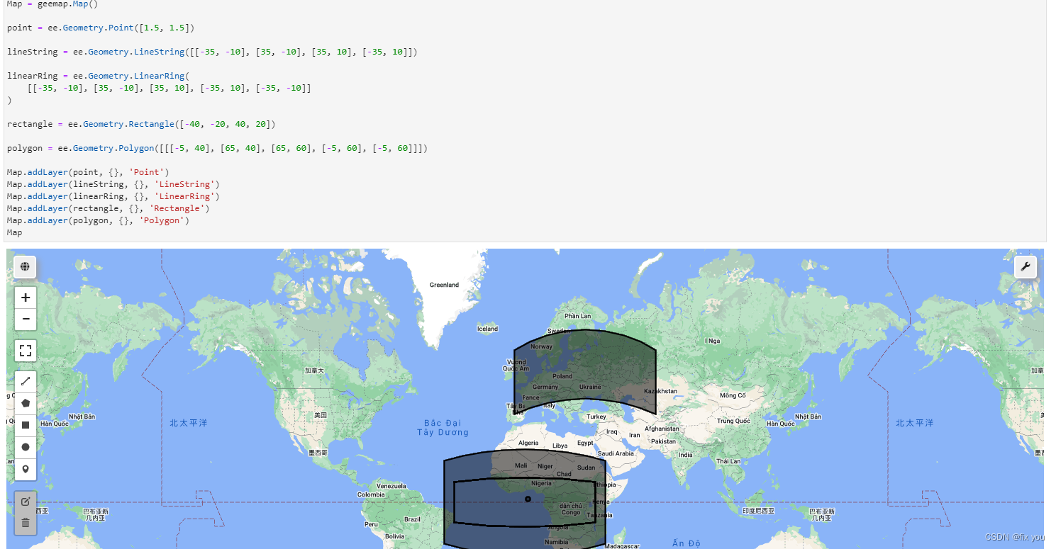
Map = geemap.Map()

point = ee.Geometry.Point([1.5, 1.5])//点

lineString = ee.Geometry.LineString([[-35, -10], [35, -10], [35, 10], [-35, 10]])//线

linearRing = ee.Geometry.LinearRing(
    [[-35, -10], [35, -10], [35, 10], [-35, 10], [-35, -10]]
)//闭合线

rectangle = ee.Geometry.Rectangle([-40, -20, 40, 20])矩形

polygon = ee.Geometry.Polygon([[[-5, 40], [65, 40], [65, 60], [-5, 60], [-5, 60]]])
//线的属性可以设置最短,那么在三维球体表面上的最短直线,在二维平铺的地图上就是曲线了.
Map.addLayer(point, {}, 'Point')
Map.addLayer(lineString, {}, 'LineString')
Map.addLayer(linearRing, {}, 'LinearRing')
Map.addLayer(rectangle, {}, 'Rectangle')
Map.addLayer(polygon, {}, 'Polygon')
Map

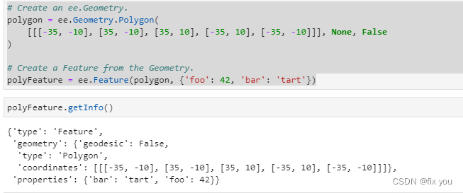
Geometry加上了属性就变成了了Feature,

# Create an ee.Geometry.
polygon = ee.Geometry.Polygon(
    [[[-35, -10], [35, -10], [35, 10], [-35, 10], [-35, -10]]], None, False
)

# Create a Feature from the Geometry.
polyFeature = ee.Feature(polygon, {'foo': 42, 'bar': 'tart'})

如图所示,我们可以看到设置在polygon上的属性

在这里插入图片描述

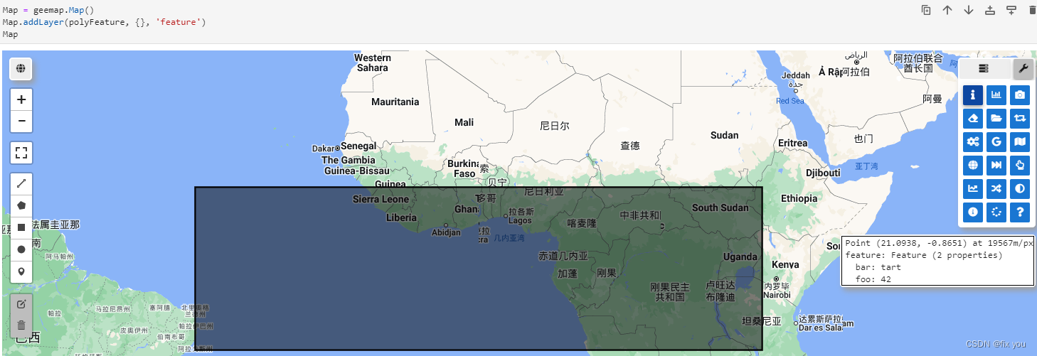
将Feature图层添加到地图上,并查看属性
在这里插入图片描述
在feature创建之后再添加属性

# Make a feature and set some properties.
feature = (
    ee.Feature(ee.Geometry.Point([-122.22599, 37.17605]))
    .set('genus', 'Sequoia')//设置键值对
    .set('species', 'sempervirens')
)

# Overwrite the old properties with a new dictionary.
newDict = {'genus': 'Brachyramphus', 'presence': 1, 'species': 'marmoratus'}//字典
feature = feature.set(newDict)

# Check the result.
feature.getInfo()

获取feature的属性

props = feature.toDictionary()
props.getInfo()
prop = feature.get('species')//根据key值获得value
prop.getInfo()

下面是一个使用的场景:
需要从一个全球的卫星遥感影像中拆解出中国的那一部分
方法如下,首先获得一个China 国界范围的featurecollection(这一步通过过滤器来实现,从featurecollection当中根据name属性筛选出来)
然后将image裁剪到featurecollection上,并将裁剪后的image图层重新加载到地图上,这里我偷懒了,截图用的是老师的.
在这里插入图片描述
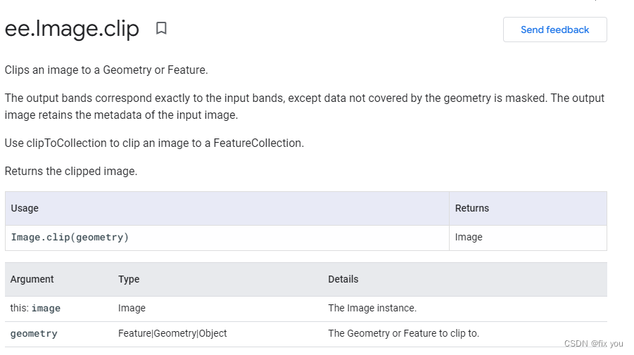
裁剪的代码:

裁剪之后的结果:

在这里插入图片描述

二、Getting image metadata

获取image的属性信息,代码如图:
在这里插入图片描述
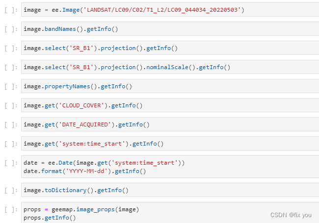
可以根据不同的代码查找到image中的不同属性值
具体的函数说明可在gee的reference当中找到
链接:https://developers.google.com/earth-engine/apidocs/ee-image

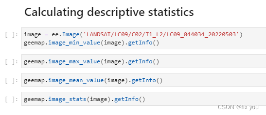
下面的还有查看影像的统计信息,类似于arcgis中查看影像的最大值最小值,这里就不在赘述.
在这里插入图片描述
另外可以方便的将JavaScript准换为Python的代码,方式如图:

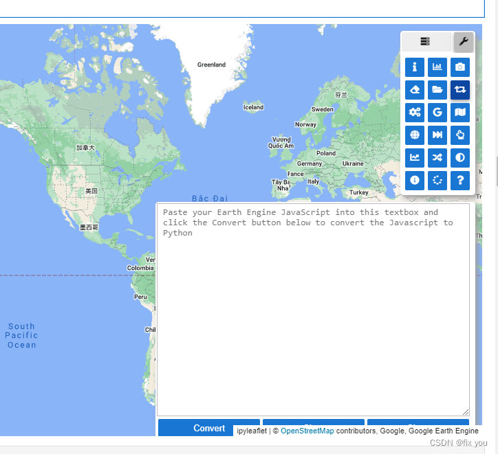
将JavaScript代码放入输入框中之后,点击convert按钮之后就会自动把代码转换为Python的格式.
当然这个转换并不是万能的只能把和gee有关的JavaScript代码进行转换,转换的结果并不保证百分之百对,需要自己注意.

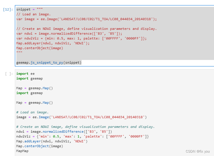
当然jupyter lab notebook 也提供了使用代码的转换方式

snippet = """
// Load an image.
var image = ee.Image('LANDSAT/LC08/C02/T1_TOA/LC08_044034_20140318');

// Create an NDWI image, define visualization parameters and display.
var ndwi = image.normalizedDifference(['B3', 'B5']);
var ndwiViz = {min: 0.5, max: 1, palette: ['00FFFF', '0000FF']};
Map.addLayer(ndwi, ndwiViz, 'NDWI');
Map.centerObject(image)
"""

geemap.js_snippet_to_py(snippet)

结果如下
在这里插入图片描述
还有批处理的方式

import os
from geemap.conversion import *

# Set the output directory
out_dir = os.getcwd()

# Set the input directory
js_dir = get_js_examples(out_dir)//定义脚本存储的位置

# Convert Earth Engine JavaScripts Python
js_to_python_dir(in_dir=js_dir, out_dir=out_dir, use_qgis=False)

# Convert Python scripts to Jupyter notebooks
py_to_ipynb_dir(js_dir)

三、Using the plotting tool和可视化

创建地图

Map = geemap.Map(center=[40, -100], zoom=4)

landsat7 = ee.Image('LANDSAT/LE7_TOA_5YEAR/1999_2003').select(
    ['B1', 'B2', 'B3', 'B4', 'B5', 'B7']
)

landsat_vis = {'bands': ['B4', 'B3', 'B2'], 'gamma': 1.4}
Map.addLayer(landsat7, landsat_vis, "Landsat")

hyperion = ee.ImageCollection('EO1/HYPERION').filter(
    ee.Filter.date('2016-01-01', '2017-03-01')
)//高光谱数据

hyperion_vis = {
    'min': 1000.0,
    'max': 14000.0,
    'gamma': 2.5,
}
Map.addLayer(hyperion, hyperion_vis, 'Hyperion')
Map

在这里插入图片描述
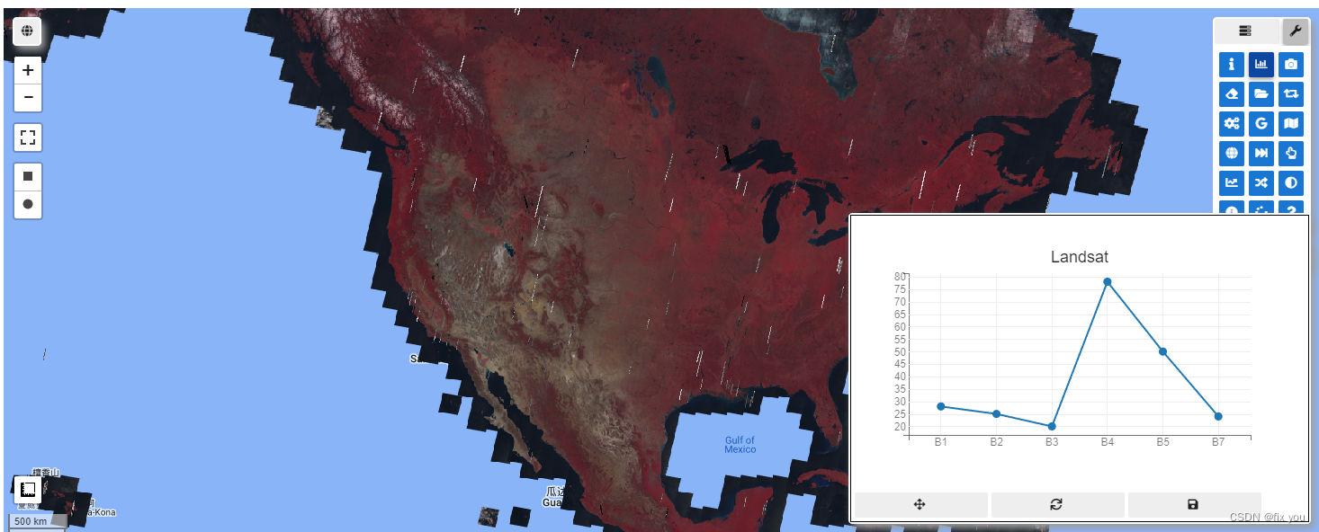
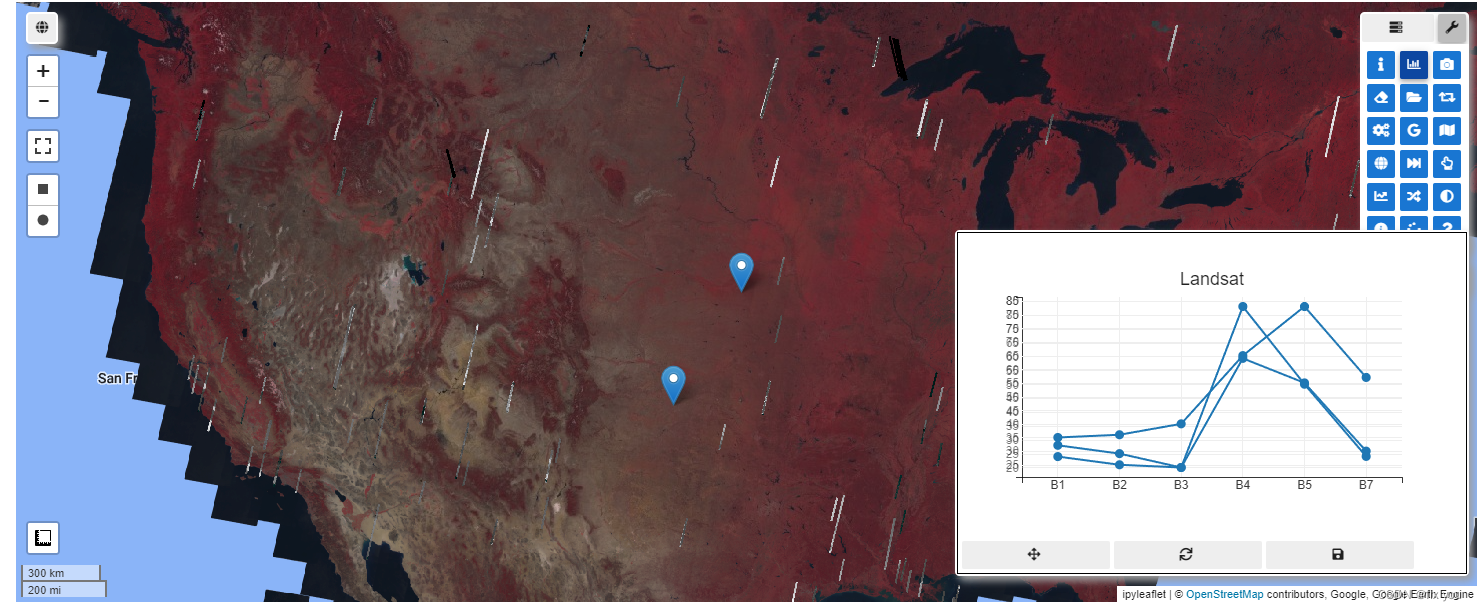
使用plotting按钮可以快速的绘制图表
Map.set_plot_options(add_marker_cluster=True, overlay=True)可以往地图上加标记点,绘制图标是会同时显示.

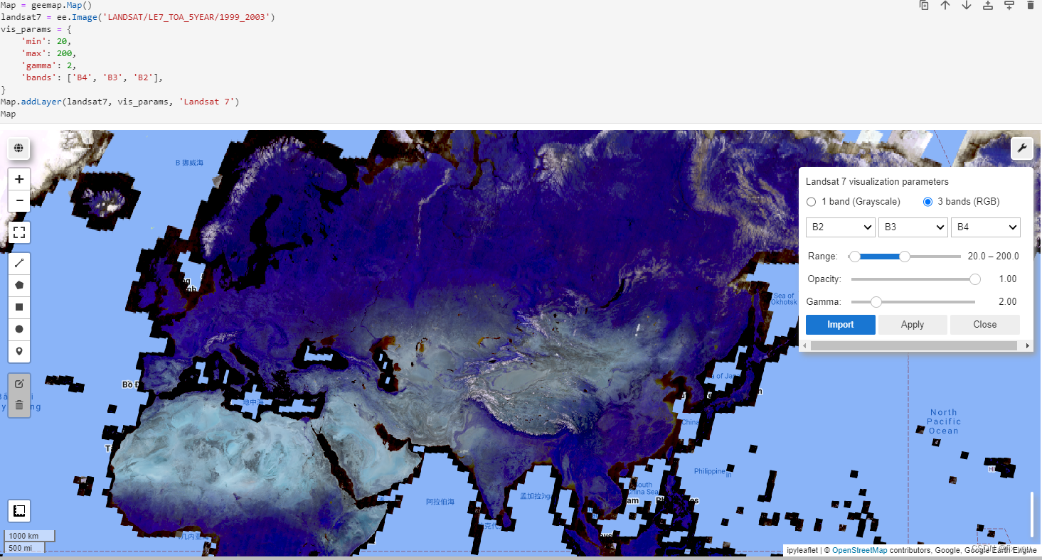
在绘图(也就是可视化)时,我们也可以通过工具来修改参数,包括最大值最小值,调色板等等.
在这里插入图片描述
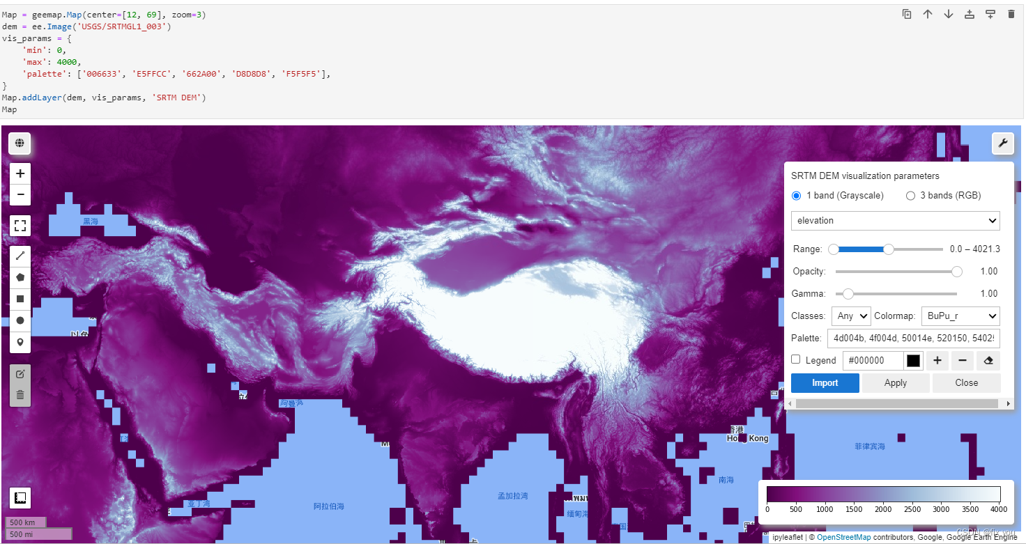
当然对于多波段数据,也可以进行多波段的合成的调整

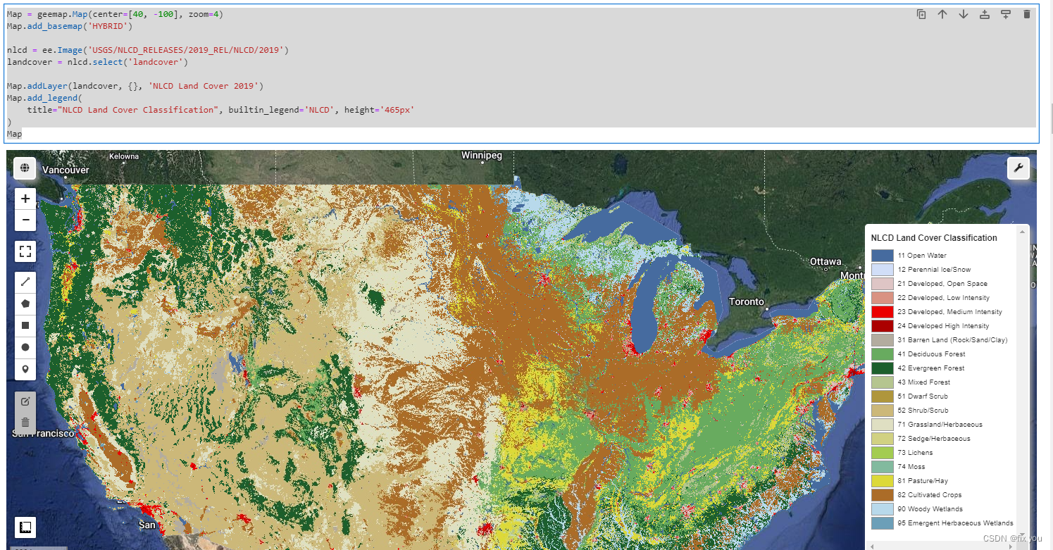
在地图上添加图例,下面是土地利用的图例:

Map = geemap.Map(center=[40, -100], zoom=4)
Map.add_basemap('HYBRID')

nlcd = ee.Image('USGS/NLCD_RELEASES/2019_REL/NLCD/2019')
landcover = nlcd.select('landcover')

Map.addLayer(landcover, {}, 'NLCD Land Cover 2019')
Map.add_legend(
    title="NLCD Land Cover Classification", builtin_legend='NLCD', height='465px'
)
Map

在这里插入图片描述
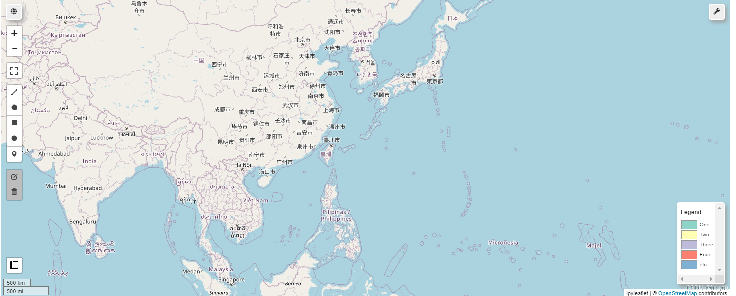
创建自己的图例

Map = geemap.Map(add_google_map=False)

legend_keys = ['One', 'Two', 'Three', 'Four', 'ect']

# colors can be defined using either hex code or RGB (0-255, 0-255, 0-255)
legend_colors = ['#8DD3C7', '#FFFFB3', '#BEBADA', '#FB8072', '#80B1D3']
# legend_colors = [(255, 0, 0), (127, 255, 0), (127, 18, 25), (36, 70, 180), (96, 68 123)]

Map.add_legend(
    legend_keys=legend_keys, legend_colors=legend_colors, position='bottomright'
)
Map

在这里插入图片描述
还有通过字典的形式:

Map = geemap.Map(center=[40, -100], zoom=4)

legend_dict = {
    '11 Open Water': '466b9f',
    '12 Perennial Ice/Snow': 'd1def8',
    '21 Developed, Open Space': 'dec5c5',
    '22 Developed, Low Intensity': 'd99282',
    '23 Developed, Medium Intensity': 'eb0000',
    '24 Developed High Intensity': 'ab0000',
    '31 Barren Land (Rock/Sand/Clay)': 'b3ac9f',
    '41 Deciduous Forest': '68ab5f',
    '42 Evergreen Forest': '1c5f2c',
    '43 Mixed Forest': 'b5c58f',
    '51 Dwarf Scrub': 'af963c',
    '52 Shrub/Scrub': 'ccb879',
    '71 Grassland/Herbaceous': 'dfdfc2',
    '72 Sedge/Herbaceous': 'd1d182',
    '73 Lichens': 'a3cc51',
    '74 Moss': '82ba9e',
    '81 Pasture/Hay': 'dcd939',
    '82 Cultivated Crops': 'ab6c28',
    '90 Woody Wetlands': 'b8d9eb',
    '95 Emergent Herbaceous Wetlands': '6c9fb8',
}

nlcd = ee.Image('USGS/NLCD_RELEASES/2019_REL/NLCD/2019')
landcover = nlcd.select('landcover')

Map.addLayer(landcover, {}, 'NLCD Land Cover 2019')
Map.add_legend(title="NLCD Land Cover Classification", legend_dict=legend_dict)
Map

需要注意:图例和地图当中的图像不是直接对应的,也就是单纯的画了个表格放到地图上而已.
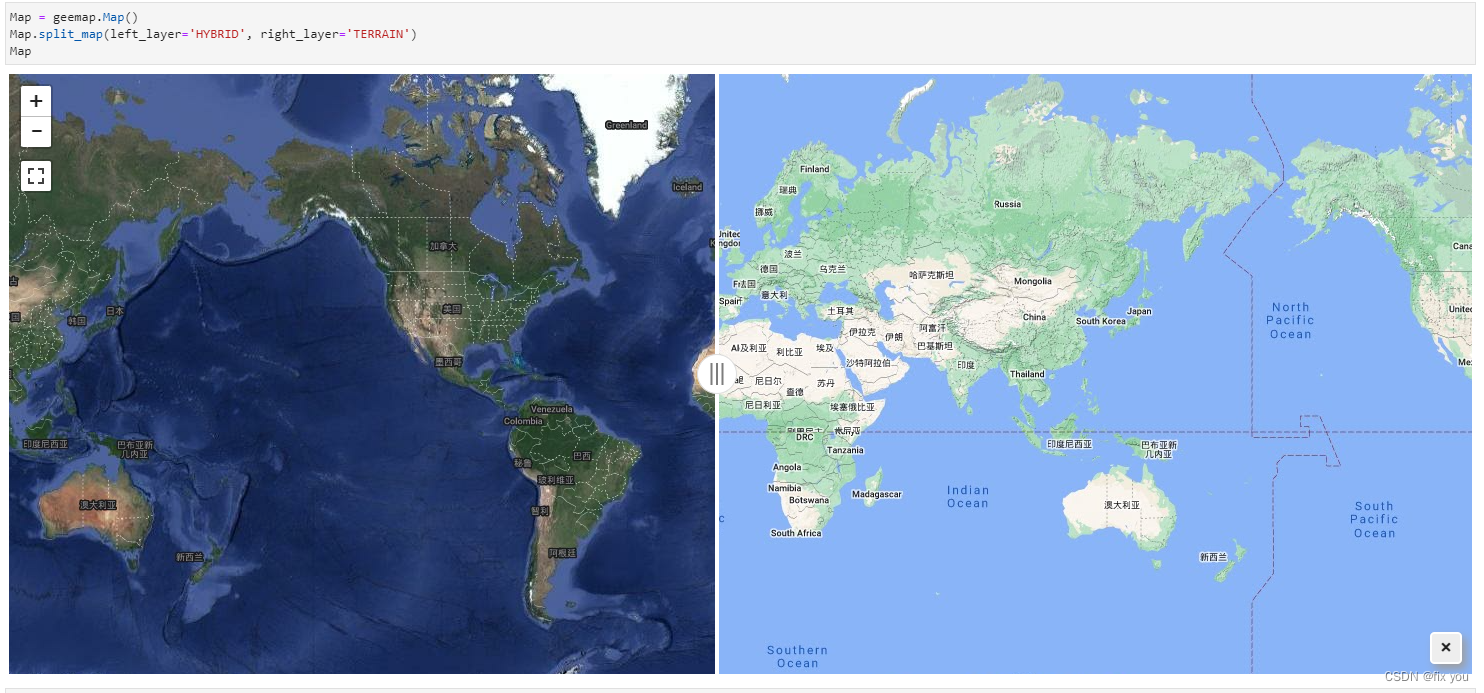
下面是Split-panel maps
效果如下,代码比较简单这里就不单独打出来了,可以把两个图层叠加到一个地图上,进行比较
在这里插入图片描述
还有四幅图一起对比比较的,而且地图互相之间联系,当其中的一幅地图发生改变时,其他的三幅也会同步发生同样的改变.

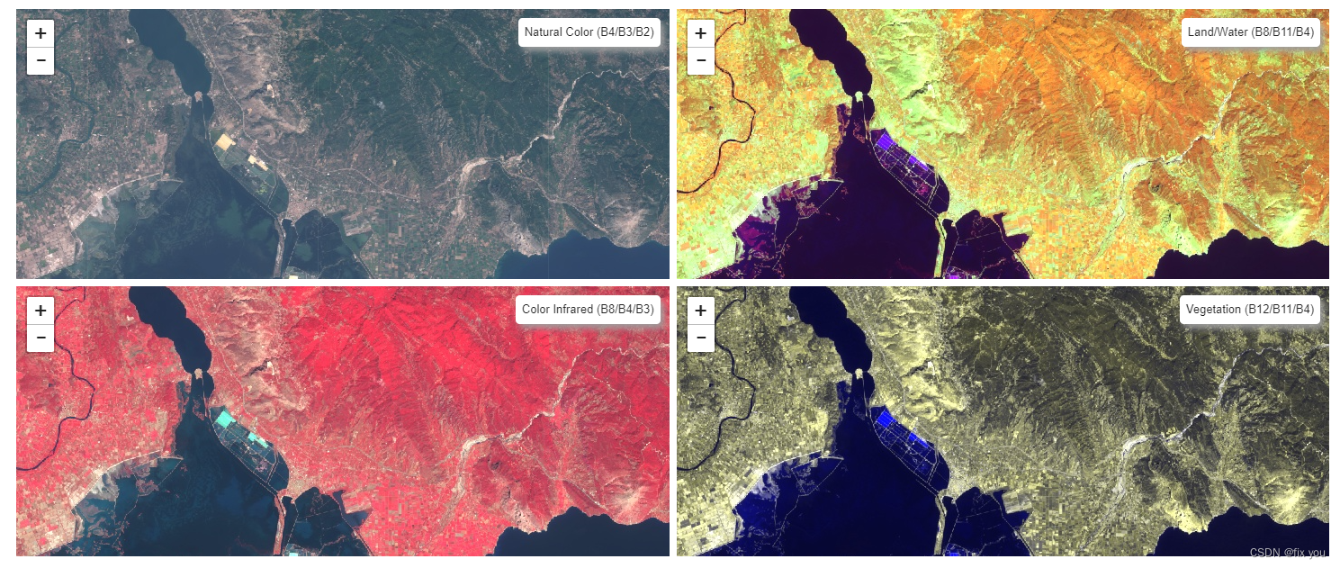
代码如下:

image = (
    ee.ImageCollection('COPERNICUS/S2')
    .filterDate('2018-09-01', '2018-09-30')
    .map(lambda img: img.divide(10000))
    .median()
)

vis_params = [
    {'bands': ['B4', 'B3', 'B2'], 'min': 0, 'max': 0.3, 'gamma': 1.3},
    {'bands': ['B8', 'B11', 'B4'], 'min': 0, 'max': 0.3, 'gamma': 1.3},
    {'bands': ['B8', 'B4', 'B3'], 'min': 0, 'max': 0.3, 'gamma': 1.3},
    {'bands': ['B12', 'B12', 'B4'], 'min': 0, 'max': 0.3, 'gamma': 1.3},
]

labels = [
    'Natural Color (B4/B3/B2)',
    'Land/Water (B8/B11/B4)',
    'Color Infrared (B8/B4/B3)',
    'Vegetation (B12/B11/B4)',
]

geemap.linked_maps(
    rows=2,
    cols=2,
    height="300px",
    center=[38.4151, 21.2712],
    zoom=12,
    ee_objects=[image],
    vis_params=vis_params,
    labels=labels,
    label_position="topright",
)

还有基于时间序列比较的模式
在这里插入图片描述
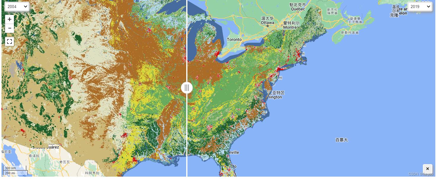
可以在地图的上方的下拉列表中选择年份,代码如下:

Map = geemap.Map(center=[40, -100], zoom=4)
collection = ee.ImageCollection('USGS/NLCD_RELEASES/2019_REL/NLCD').select('landcover')
vis_params = {'bands': ['landcover']}
years = collection.aggregate_array('system:index').getInfo()
years
Map.ts_inspector(
    left_ts=collection,
    right_ts=collection,
    left_names=years,
    right_names=years,
    left_vis=vis_params,
    right_vis=vis_params,
    width='80px',
)
Map