IOMiner: Large-scale Analytics Framework for Gaining Knowledge from I/O Logs

Modern HPC systems are collecting large amounts of I/O performance data. The massive volume and heterogeneity of this data, however, have made timely performance of in-depth integrated analysis difficult. To overcome this difficulty and to allow users to identify the root causes of poor application I/O performance, we present IOMiner, an I/O log analytics framework. IOMiner provides an easy-touse interface for analyzing instrumentation data, a unified storage schema that hides the heterogeneity of the raw instrumentation data, and a sweep-line-based algorithm for root cause analysis of poor application I/O performance.IOMiner is implemented atop Spark to facilitate efficient, interactive, parallel analysis. We demonstrate the capabilities of IOMiner by using it to analyze logs collected on a largescale production HPC system. Our analysis techniques not only uncover the root cause of poor I/O performance in key application case studies but also provide new insight into HPC I/O workload characterization.

现代HPC系统正在收集大量的I/O性能数据。然而，这些数据的庞大数量和异构性给及时进行深度综合分析带来了困难。为了克服这个困难并允许用户识别应用程序I/O性能差的根本原因，我们提出了IOMiner，一个I/O日志分析框架。IOMiner提供了一个易于使用的接口来分析仪器数据，一个统一的存储模式来隐藏原始仪器数据的异构性，以及一个基于扫描线的算法来分析应用程序I/O性能差的根本原因。IOMiner在Spark之上实现，以促进高效、交互式、并行的分析。通过使用IOMiner分析在大规模生产HPC系统上收集的日志，我们演示了IOMiner的功能。我们的分析技术不仅揭示了关键应用程序案例研究中I/O性能差的根本原因，而且还为HPC I/O工作负载表征提供了新的见解。

数据异构性（The heterogeneity of this data）。数据异构指的是在一个系统或环境中存在多种不同类型、格式或结构的数据。这些数据可能来自不同的源头，具有不同的组织方式、语义定义、编码规范或存储形式。数据异构性在现代的信息系统中很常见，原因包括：
1.数据源多样性：不同的数据源可能使用不同的数据模型、数据库管理系统或应用程序，导致数据的结构和格式差异。
2.数据存储和交换的多样性：数据可能存储在各种不同的数据库、文件格式或数据存储系统中，例如关系型数据库、NoSQL数据库、平面文件、XML文件等。
3.数据集成和集成系统的复杂性：在数据集成过程中，需要将来自不同数据源的数据进行合并、转换和映射，以实现数据的一致性和可用性。
4.数据异构性对数据管理和分析带来了挑战，因为不同类型的数据需要使用特定的工具和技术进行处理。为了处理数据异构性，通常需要进行数据清洗、转换和标准化，以便在分析和应用中能够使用这些数据。

仪器数据（instrumentation data）。仪器数据是指从仪器或传感器中收集的数据，用于测量和监测系统或过程中的各种物理或操作参数。它常用于工程、科学、制造和研究等领域。仪器数据可以来自多种来源，包括：
1.传感器：各种类型的传感器，如温度传感器、压力传感器、流量传感器、振动传感器等，根据设计的物理或环境条件收集数据。
2.控制系统：仪器数据可以从监测和调节过程或设备的控制系统中获取。这些系统通常提供与操作参数、控制信号和系统状态相关的数据。
3.测试和测量设备：用于测试和测量的仪器，如示波器、光谱仪、数据记录仪和信号分析仪，在实验、检查或性能评估过程中生成仪器数据。
4.收集的仪器数据通常包括数值测量、时间戳和其他相关元数据。这些数据通常存储在数据库或数据存储库中，以供进一步分析、可视化和决策使用。它可以提供有关系统性能的有价值信息，识别异常或故障，实现预测性维护，优化流程，并支持科学研究。

I. INTRODUCTION

Parallel I/O is a crucial component for handling massive data movement on high-performance computing (HPC) systems. In an effort to characterize, understand, and eventually optimize parallel I/O performance of applications, I/O logs are captured at several stages of the I/O path. At the application level, instrumentation tools such as Darshan [1], [2] collect detailed I/O statistics. Darshan stores the data in a write-optimized format; for example, each MPI job produces a compressed binary log file. The number of Darshan logs produced on production HPC systems each month depends on the number of executed jobs , and the data volume ranges from hundreds of gigabytes to multiple terabytes.File-system-monitoring tools, such as the Lustre Monitoring Tool (LMT) [3], periodically gather I/O load on file system servers and store the traces either in files or in databases. The frequency of file system instrumentation is a few seconds, resulting in tens of thousands of records per day. In addition, job schedulers such as Slurm [4] can log millions of jobs’ resource utilization each month, such as the compute nodes used and the jobs’ execution times.

并行I/O是在高性能计算(HPC)系统上处理大量数据移动的关键组件。为了描述、理解并最终优化应用程序的并行I/O性能，在I/O路径的几个阶段捕获I/O日志。在应用程序级别，Darshan[1]、[2]等工具收集详细的I/O统计信息。Darshan以写优化格式存储数据；例如，每个MPI作业生成一个压缩的二进制日志文件。每个月生产HPC系统上产生的Darshan日志数量取决于执行的作业数量，数据量从数百gb到多个tb不等。文件系统监控工具，如Lustre Monitoring Tool (LMT)[3]，定期收集文件系统服务器上的I/O负载，并将跟踪记录存储在文件或数据库中。文件系统检测的频率是几秒，导致每天有数以万计的记录。此外，Slurm[4]等作业调度器每月可以记录数百万个作业的资源利用率，例如使用的计算节点和作业的执行时间。

An integrated analysis of all I/O instrumentation data faces several challenges. First, instrumentation tools provide ad hoc interfaces for data extraction, requiring tedious manual effort in resolving their incompatibilities. Second, instrumentation tools often store data in write-optimized format, making analytics on such formats inefficient.

对所有I/O仪表数据进行集成分析面临几个挑战。首先，仪表工具提供用于数据提取的AD hoc临时接口，需要繁琐的手工工作来解决它们的不兼容性。其次，检测工具通常以写优化格式存储数据，使得对这种格式的分析效率低下。

Write-optimized格式是一种旨在提高写入性能的数据存储格式。它主要关注数据的写入操作，并采用特定的设计和优化策略来减少写入开销、提高写入吞吐量和降低写入延迟。以下是一些常见的Write-optimized格式的特点和技术：
1.日志结构（Log-Structured）：Write-optimized格式通常采用日志结构的存储方式，其中所有的写入操作都追加到日志中。这种方式避免了在更新现有数据时的随机写入，而是将写入操作集中在顺序追加的日志中。
2.批量写入（Batch Writes）：Write-optimized格式倾向于批量写入数据，而不是单个记录的逐个写入。通过将多个写入操作打包成批量写入，可以减少写入操作的开销，例如磁盘寻址和索引更新。
3.写缓冲（Write Buffering）：Write-optimized格式使用写缓冲来缓存写入操作，并在适当的时机进行合并和排序。这样可以减少磁盘写入次数，提高写入效率。
4.压缩（Compression）：Write-optimized格式通常采用压缩算法来减少写入数据的存储空间。压缩可以降低磁盘写入开销，并提高存储容量利用率。
5.写入顺序优化（Write Order Optimization）：Write-optimized格式会优化写入顺序，使得相邻的写入操作能够尽可能地集中在一起，从而减少磁盘的寻址和旋转延迟。
6.写前日志（Write-Ahead Log）：Write-optimized格式使用写前日志，即在写入数据之前先将操作记录到日志中。这种方式可以保证数据的一致性和持久性，并提供容错和恢复机制。
7.垃圾收集（Garbage Collection）：Write-optimized格式通常使用垃圾收集机制，定期清理和回收不再需要的数据。垃圾收集可以释放空间，维护数据结构的一致性，并提高读取性能。
通过这些优化策略和技术，Write-optimized格式能够提供高效的写入性能和较低的写入延迟。这使得它们在需要频繁写入数据的场景中非常有用，例如日志记录、实时数据处理和数据库系统等。

In general, analysis has relied on manually written scripts, a time-consuming process with limited portability. Another option is to load data into a database and apply SQL queries.We have previously analyzed multilevel and multiplatform I/O logs by loading data into a MySQL database [5].However, the performance of data analytics can be limited by the single database server and parallel databases on HPC system are rarely installed

一般来说，分析依赖于手工编写的脚本，这是一个耗时且可移植性有限的过程。另一种选择是将数据加载到数据库中并应用SQL查询。我们以前通过将数据加载到MySQL数据库中来分析多级和多平台I/O日志[5]。然而，数据分析的性能受到单一数据库服务器的限制，HPC系统上很少安装并行数据库。

As a step toward solving the challenges of analyzing multilevel I/O instrumentation data that is massive in size and heterogeneous, and allowing users to easily identify the root causes of poor I/O performance from the complex instrumentation data, we introduce the IOMiner framework.The main components of IOMiner are an extensible set of unified interfaces that can be used to compose common I/O analysis operations on multilevel instrumentation data, a query-friendly and unified storage schema that hides the heterogeneity of different schema of instrumentation data and is optimized for parallel analytics on HPC, and a sweep-line-based [6] analysis function that helps users easily identify the root causes for an application’s poor I/O performance. The IOMiner framework is built on Apache Spark [7], enabling interactive and ad hoc querying and statistical analysis.

为了解决分析规模庞大且异构的多级I/O检测数据的挑战，并允许用户从复杂的检测数据中轻松识别I/O性能差的根本原因，我们引入了IOMiner框架。IOMiner的主要组件是一组可扩展的统一接口，可用于对多级仪器仪表数据进行通用I/O分析操作;一个查询友好的统一存储模式，它隐藏了仪器仪表数据不同模式的异质性，并针对HPC上的并行分析进行了优化;一个基于扫描线的[6]分析功能，可帮助用户轻松识别应用程序I/O性能差的根本原因。IOMiner框架建立在Apache Spark上[7]，支持交互式和临时查询和统计分析。

The main contributions of this paper are as follows.

• A set of unified interfaces that can be used to compose the first-order and in-depth data analysis of different types of instrumentation data
• A query-friendly and unified storage schema that fuses together different instrumentation data and loads logs on demand based on the analysis to be performed
• A layout-aware data placement and task-dispatching framework for parallel data analytics using Spark. Both data placement and task dispatching are specialized for HPC storage architecture
• A sweep-line analysis function that helps identify the root causes for an application’s poor I/O performance

本文的主要贡献如下。

• 一套统一的接口，可用于对不同类型的仪器仪表数据进行一阶深度数据分析
• 查询友好的统一存储模式，将不同的检测数据融合在一起，并根据要执行的分析按需加载日志
• 一个布局感知的数据放置和任务调度框架，用于使用Spark进行并行数据分析。数据放置和任务调度都是专门为HPC存储架构设计的
• 一种扫描线分析功能，可帮助确定导致应用程序I/O性能差的根本原因

一阶数据分析（First-order data analysis）指的是对原始数据进行初步检查和总结，以获得对数据集的基本理解。它涉及基本的统计量和探索性数据分析技术，用于描述数据并识别任何显著的模式或趋势。一阶分析通常关注描述性统计，如均值、中位数、众数、标准差、范围和频率分布等。
深度数据分析（In-depth data analysis）则超越了表面层次的检查，更详细地探索数据。它涉及应用高级统计技术和更复杂的方法，以揭示数据集中隐藏的洞察、关系和模式。深度分析的目标是更深入地理解数据，提供更全面和有意义的见解。

We have evaluated IOMiner’s capabilities to support both first-order and more in-depth analysis. Our analysis ranges from the distribution of the sequential I/O, per job read/write ratio, and usage of the customized striping configuration, to the usage of different I/O middleware and the composition of various file-sharing patterns. Our analysis provides valuable insights for both system administrators and I/O specialists. Our analyses with IOMiner also include the root cause identification using the sweep-line technique for jobs experiencing poor I/O bandwidth.

我们已经评估了IOMiner支持一阶和更深入分析的能力。我们的分析范围从顺序I/O的分布、每个作业的读/写比率、自定义条分层配置的使用，到不同I/O中间件的使用和各种文件共享模式的组成。我们的分析为系统管理员和I/O专家提供了有价值的见解。我们对IOMiner的分析还包括使用扫描线技术对I/O带宽差的作业进行根本原因识别。

数据分层配置（striping configuration）是计算机存储系统中的一种技术，用于将数据分散存储在多个存储设备或磁盘中。它通常在RAID（独立磁盘阵列）系统中使用，以提高性能和可靠性。在数据分层配置中，数据被分割成小的片段（或称为"stripes"），每个片段被写入存储系统中的不同磁盘中。通过将数据分布在多个磁盘上，系统可以进行并行的读写操作，从而提高整体吞吐量并降低延迟。

The remainder of the paper is organized as follows. We present the IOMiner framework including the interfaces, storage schema, Spark-based implementation, and approach for analyzing the root causes of poor I/O performance in Section II. In Section III, we evaluate IOMiner capabilities, and in Section IV, we discuss related work. We conclude in Section V with a brief discussion of future work.

本文的其余部分组织如下。在第二节中，我们介绍了IOMiner框架，包括接口、存储模式、基于spark的实现以及分析I/O性能差的根本原因的方法。在第三节中，我们将评估IOMiner的能力，在第四节中，我们将讨论相关工作。最后，我们在第五节简要讨论今后的工作。

II. DESIGN OF IOMINER

A. Unified Query Interfaces for I/O Log Analytics

To simplify users’ effort and to make IOMiner flexible and efficient for handling queries, we have designed IOMiner with a set of interfaces applicable to different log types (e.g., Darshan, Slurm, and LMT). These interfaces include sort, group, filter, project, and join, which are all common to SQL. IOMiner also provides additional operators (e.g., percentile and bin) that are often used for I/O log analytics. IOMiner further complements the functions of the existing interfaces with support for user-defined functions, thus allowing users to flexibly express complex queries. All of these interfaces are layered on top of Spark, allowing the output of one operator to be supplied as the input of another operator using Spark RDD (resilient distributed dataset).

为了简化用户的工作，并使IOMiner灵活高效地处理查询，我们为IOMiner设计了一组适用于不同日志类型（例如，Darshan、Slurm和LMT）的接口。这些接口包括排序、组、筛选、项目和连接，这些都是SQL中常见的。IOMiner还提供了额外的操作符（例如，百分位数和bin），这些操作符通常用于I/O日志分析。IOMiner通过支持用户定义函数进一步补充了现有接口的功能，从而允许用户灵活地表达复杂的查询。所有这些接口都是在Spark之上分层的，允许使用Spark RDD（弹性分布式数据集）将一个操作符的输出作为另一个操作符的输入提供。

Algorithm 1 gives an overview of how to use IOMiner.

Line 14 returns a list of tuples containing the jobs whose write sizes are smaller than 1 GB. This analysis is satisfied by a pipeline of operators stitched together. In line 15, the user-defined function classify workload bins each tuple of job tuples based on bytes written (e.g., [0 − 1) GB is workload 0, [1, 10) GB is workload 1, [10, ∞) GB is workload 2). These bin values are tagged to each element in job tuples as a new field “workload.” In line 17, the user-defined function calculate ost count accepts file tuples grouped by job id and calculates the number of distinct OSTs for each job. In line 19, the percentile operator sorts selected tuples by bytes written and returns a percentile list for bytes written. It answers queries like “What is the distribution of write sizes across all the jobs?”

算法1概述了如何使用IOMiner。第14行返回一个元组列表，其中包含写大小小于1GB的作业。这种分析通过连接在一起的操作符流水线来实现。在第15行，用户定义的函数根据写入的字节对工作元组中的每个元组的工作负载进行分类(例如，[0−1)GB是工作负载0，[1,10)GB是工作负载1，[10，∞)GB是工作负载2)。这些bin值作为新字段“workload”标记到工作元组中的每个元素上。在第17行，用户定义的函数calculate ost count接受按作业id分组的文件元组，并计算每个作业的不同ost的数量。在第19行，百分位运算符按写入的字节对所选元组进行排序，并返回写入字节的百分位列表。它会回答诸如“所有作业的写大小分布如何?”

Algorithm 1: Example analysis code using IOMiner
1 # Instantiate an IOMiner instance
2 miner = IOMiner(“setup.json”)
3 # construct IOMiner’s storage format
4 miner.init stores(start date, end date)
5 # load Darshan’s job-level statistics as tuples
6 job tuples = miner.load(“darshan job”)
7 # load Darshan’s file-level statistics
8 file tuples = miner.load(“darshan file”)
9 # load Slurm job scheduler statistics
10 slurm tuples = miner.load(“slurm”)
11 # load Lustre Monitoring Tools (LMT) traces
12 lmt tuples = miner.load(“lmt”)
13 # filter jobs that write less than 1GB data and bin them
14 selected tuples = job tuples.project(“job id”,“bytes written”).filter(“bytes written < 1GB”)
15 binned tuples = job tuples.bin(“workload”,classify workload, “bytes written”)
16 # select a list of tuples containing each job’s ID and the number of Lustre storage targets (OSTs) used
17 grouped tuples = file tuples.group(“job id”,calculate ost count)
18 # generate a percentile list for Bytes Written
19 percents = job tuples.percentile(“bytes written”)
20 # return each job’s node count (in Slurm log) and and write/read size (in Darshan log)
21 joined tuples = job tuples.join(slurm tuples,“job id”).project(“job id”, “node count”,“bytes read”, “bytes written”)
22 # return the jobs that write more than 10GB data
23 low bw tuples = job tuples.filter(“bytes written > 10GB”).join(file tuples, “job id”)
24 # extract contributing factors for poor write performance
25 perf factors = low bw tuples.extract perf factors(“0”,“1GB”, “write”)

B. Query-Friendly Storage Schema

A unified set of query interfaces eases users’ effort in defining analytic functions.Various challenges arise in providing efficient execution of these functions because of distinct characteristics of instrumentation data.For example, existing instrumentation tools generally provide vendorspecific interfaces, and it is nontrivial to implement the same function multiple times based on the interfaces of each instrumentation tool.Moreover, the storage schema of existing instrumentation tools are not designed to efficiently support analytics and query patterns.Mining results from their individual formats can incur heavy overheads.For instance, Darshan produces one log file for each job, which can be parsed by Darshan utility into a human-readable log file containing both coarse-grained job-level statistics,such as the total number of reads issued by all processes in the job, as well as fine-grained file-level statistics,such as the total number of reads issued on each file.These two types of statistics are stored in two different regions of the log file.For a query that requires a scan of all job-level and filelevel statistics, an analysis framework has to open/close all the jobs’ log files and to perform repeated seek operations inside each log to extract all the requested information.Answering this query incurs substantial metadata access (with file open/close) and file seek overhead, since Darshan can produce millions of logs in a month.

一组统一的查询接口简化了用户定义分析函数的工作。由于仪器仪表数据的不同特性，在提供这些功能的有效执行方面出现了各种各样的挑战。例如，现有的仪器工具通常提供特定于供应商的接口，并且基于每个仪器工具的接口多次实现相同的功能是很重要的。此外，现有检测工具的存储模式并不能有效地支持分析和查询模式。从它们各自的格式中挖掘结果可能会带来沉重的开销。例如，Darshan为每个作业生成一个日志文件，Darshan utility可以将其解析为包含粗粒度作业级统计信息的人可读日志文件，例如作业中所有进程发出的读操作总数，以及细粒度的文件级统计信息，例如对每个文件发出的读取总数。
这两种类型的统计信息存储在日志文件的两个不同区域。对于需要扫描所有作业级和文件级统计信息的查询，分析框架必须打开/关闭所有作业的日志文件，并在每个日志中执行重复的seek操作，以提取所有请求的信息。回答这个查询需要大量的元数据访问(打开/关闭文件)和文件查找开销，因为Darshan可以在一个月内生成数百万条日志。

To address these challenges, we have designed a unified storage schema that abstracts away the format difference between diverse instrumentation tools and is query-friendly. In Figure 1, the statistics of different instrumentation tools are formatted as tables and stored as separate files. Formatting happens when the users instantiate an IOMiner instance and invoke init stores to convert logs produced during a given time period (Line 4 of Algorithm 1); only statistics in logs of that period are extracted and reshaped into IOMiner’s storage format. This formatting operation happens only once.Later operations for the same time period will not repeat this formatting process if these tables already exist. In Figure 1, the formatted tables can be connected with each other based on specific fields. For instance, the Slurm table contains job statistics (e.g., number of cores/nodes used in a job) supplementary to Darshan’s per job statistics, so tuples in the Slurm table can be associated with Darshan tables using job id. On the other hand, LMT tables contain the systemwide read/write size for each OST during each 5-second interval (see Figure 1); the Darshan file table also contains the OST list for each file and the corresponding I/O timing.Associating these two types of logs based on OSTs and I/O time allows users to derive valuable insights, such as how I/O operations on one file are interfered with by other I/O operations being serviced on the same set of OSTs.

为了应对这些挑战，我们设计了一个统一的存储模式，它抽象了不同工具之间的格式差异，并且对查询友好。在图1中，不同检测工具的统计数据被格式化为表，并存储为单独的文件。当用户实例化IOMiner实例并调用init stores来转换给定时间段内生成的日志时，就会进行格式化(算法1的第4行);只有该时间段的日志中的统计信息被提取并重塑为IOMiner的存储格式。此格式化操作只发生一次。如果这些表已经存在，同一时间段的后续操作将不会重复此格式化过程。在图1中，格式化的表可以基于特定字段相互连接。例如，Slurm表包含Darshan的每个作业统计数据的补充作业统计数据(例如，一个作业中使用的核心/节点数)，因此Slurm表中的元组可以使用作业id与Darshan表相关联。另一方面，LMT表包含每个OST在每5秒间隔内的系统范围的读/写大小(参见图1);Darshan文件表还包含每个文件的OST列表和相应的I/O定时。根据ost和I/O时间将这两种类型的日志关联起来，使用户可以获得有价值的见解，例如，在同一组ost上提供服务的其他I/O操作如何干扰一个文件上的I/O操作。

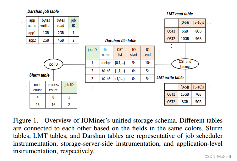
In order to avoid the excessive metadata access and file seek overheads of using Darshan’s format, IOMiner combines the job-level statistics of all Darshan logs into a single table (Darshan job table in Figure 1).IOMiner does the same for the file-level statistics and stores them into a separate table (Darshan file table in Figure 1). All tuples in these tables are ordered by job id. By extracting the statistics from Darshan’s individual job logs and storing them in two tables, a query based on a given condition (e.g., bytes written < 1GB) does not have to scan through all the job logs and thus avoids the repeated open/close overhead. On the other hand, separating the job-level and file-level statistics into two tables more efficiently answers the queries performed exclusively on job-level and file-level statistics. For instance, answering a query that could be satisfied by the job-level statistics does not have to scan the file-level statistics if they are separated. In order to accelerate analytics based on the file system (Lustre in this case) information, IOMiner stores the list of storage targets (Lustre OSTs) used for each file access as a bitmap (shown in the Darshan file table in Figure 1). With this design choice, users can easily calculate the OST count used by each job by performing a union operation on all bitmaps of its files. They can also find the OSTs used by a selected set of jobs by performing intersection operations on the bitmaps of each job.

为了避免使用Darshan格式带来的过多元数据访问和文件查找开销，IOMiner将所有Darshan日志的作业级统计信息合并到一个表中(图1中的Darshan作业表)。对文件级统计数据执行相同的操作，并将它们存储到一个单独的表中(图1中的Darshan文件表)。这些表中的所有元组都按作业id排序。通过从Darshan的单个作业日志中提取统计信息并将其存储在两个表中，基于给定条件(例如，写入的字节数< 1GB)的查询不必扫描所有作业日志，从而避免了重复的打开/关闭开销。另一方面，将作业级和文件级统计信息分离到两个表中可以更有效地回答只对作业级和文件级统计信息执行的查询。例如，回答可以由作业级统计信息满足的查询时，如果文件级统计信息是分开的，则不必扫描它们。为了加速基于文件系统(本例中为Lustre)信息的分析，IOMiner将用于每个文件访问的存储目标列表(Lustre OST)存储为位图(如图1中的Darshan文件表所示)。使用这种设计选择，用户可以通过对其文件的所有位图执行联合操作来轻松计算每个作业使用的OST计数。它们还可以通过对每个作业的位图执行交集操作来找到一组选定作业所使用的ost。

C.基于spark的HPC环境实现

The storage schema mentioned in Section II-B is best suited to running analytics operations using a single process, since only one or two tables are constructed for each log type (i.e., one for Slurm, two for Darshan, as shown in Figure 1).However, supercomputers can run as many as millions of jobs each month. Since Slurm and Darshan create one or multiple long tuples for each job, mining useful information from their tables using a single process is time-consuming.To accelerate data analysis, IOMiner uses parallel processing implemented with PySpark, a Python API for the Spark framework. In PySpark, the driver process splits data into multiple partitions and parallelizes data analytics by dispatching tasks to multiple executors. Since HPC adopts a different storage architecture from the cloud computing environment [8], where Spark is typically used, we have designed a specialized data layout and task-dispatching mechanism for Spark on HPC, which parallelizes the dataloading operations from the storage servers (e.g., OST for Lustre) in a layout-aware manner.

第II-B节中提到的存储模式最适合使用单个进程运行分析操作，因为每种日志类型只构建一个或两个表(例如，一个用于Slurm，两个用于Darshan，如图1所示)。然而，超级计算机每个月可以运行多达数百万个任务。由于Slurm和Darshan为每个作业创建一个或多个长元组，因此使用单个进程从它们的表中挖掘有用的信息非常耗时。为了加速数据分析，IOMiner使用PySpark实现的并行处理，PySpark是Spark框架的Python API。在PySpark中，驱动进程将数据分成多个分区，并通过将任务分配给多个执行器来并行化数据分析。由于HPC采用的存储架构不同于云计算环境[8]，而云计算环境通常使用Spark，因此我们为HPC上的Spark设计了一种专门的数据布局和任务调度机制，以一种布局感知的方式并行处理来自存储服务器(例如，OST for Lustre)的数据加载操作。

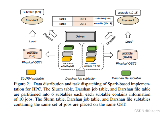
Figure 2 shows this data layout. The Darshan job table, Darshan file table, and Slurm table are split into the same number of subtables. Each subtable is placed on one OST as a separate file, and IOMiner intentionally balances the number of subtables on each OST. In doing so, it also places Darshan files and Slurm files that contain the same set of jobs on the same OSTs. For instance, in Figure 2, three Slurm subtables, Darshan job subtables, and Darshan file subtables belonging to Job [1–30] and [31–60] are placed on OST1 and OST2, respectively. In this way, each OST contains 9 subtables belonging to the same set of jobs, and a joining operator based on job id does not incur data traffic on additional OSTs, isolating each executor’s traffic on one OST without competing for other OST’s bandwidth.

图2显示了这个数据布局。Darshan作业表、Darshan文件表和Slurm表被分成相同数量的子表。每个子表作为单独的文件放在一个OST上，并且IOMiner有意平衡每个OST上的子表数量。在此过程中，它还将包含相同作业集的Darshan文件和Slurm文件放在相同的ost上。例如，在图2中，属于job[1-30]和[31-60]的三个Slurm子表、Darshan作业子表和Darshan文件子表分别放在OST1和OST2上。这样，每个OST包含属于同一组作业的9个子表，并且基于作业id的连接操作符不会在额外的OST上产生数据流量，将每个执行器的流量隔离在一个OST上，而不会竞争其他OST的带宽。

D. Sweep-line-based Root Cause Analysis of Poor I/O Performance

Analyzing an application’s poor I/O performance has been a common effort of both the application developers and the system administrators. However, existing approaches are generally based on manual profiling; no easy approach has been devised that can filter applications with poorI/O performance from a massive set of logs and provide insightful feedback to the users.

分析应用程序糟糕的I/O性能一直是应用程序开发人员和系统管理员的共同工作。然而，现有的方法通常是基于手动分析；目前还没有一种简单的方法可以从大量日志中过滤出i /O性能较差的应用程序，并向用户提供有洞察力的反馈。

To fill this void, we designed IOMiner to mine the instances of poorly performing I/O from logs and to identify how different contributing factors to performance are playing a role: in Line 23-25 of Algorithm 1, the extract perf factors function returns a list of tuples, where each tuple includes the values of a set of key performance-contributing factors to each job whose write bandwidth is between 0 and 1GB/s. We currently consider the following five common contributing factors in IOMiner：

• Small I/O requests (Small) – The percentage of small I/O requests among all the I/O requests: A large number incurs longer time for writing/reading data to/from disks because of slow file seek performance.
• Nonconsecutive I/O requests (Non-consec) – The percentage of noncontiguous I/O requests: I/O requests that are not requesting consecutive byte streams result in small and random I/O requests to the file system.
• Utilization of collective I/O (Coll): A value of 0 or 1 that indicates whether collective I/O has been used in a job. A job using collective I/O typically optimizes its read/write operations by transforming the small, nonconsecutive I/O into fewer larger ones.
• Number of OSTs used by each job (OST#): The total number of distinct OSTs used by a job. A large value means that a job uses more storage resource.
• Contention level (Proc/OST): The ratio of the process count accessing a file to the file’s stripe count. A high value implies that a large number of processes are competing for the same OSTs’ bandwidth

为了填补这一空白，我们设计了IOMiner来从日志中挖掘性能较差的I/O实例，并确定影响性能的不同因素是如何发挥作用的:在算法1的第23-25行中，extract perf factors函数返回一个元组列表，其中每个元组包含一组关键性能影响因素的值，这些因素适用于写带宽在0到1GB/s之间的每个作业。我们目前考虑IOMiner中的以下五个常见影响因素：

• 小I/O请求(Small)———小I/O请求占所有I/O请求的百分比:数量太多会导致从磁盘读写数据的时间变长，因为文件寻道性能变慢。
• 不连续I/O请求(Non-consec)——不连续I/O请求的百分比：不请求连续字节流的I/O请求会导致对文件系统的小且随机的I/O请求。
• 集合I/O利用率(Coll)：取值为0或1，表示作业中是否使用了集合I/O。使用集合I/O的作业通常通过将小的、非连续的I/O转换为更少的大I/O来优化其读/写操作。
• 每个作业使用的OST数量(OST#)：一个作业使用的不同OST的总数。值越大，表示作业占用的存储资源越多。
• 争用级别(Proc/OST):访问文件的进程数与文件的条带数之比。该值越高，表示有大量进程在竞争同一个ost的带宽。

While these factors are considered as the common reasons for an application’s low I/O performance, we believe there can be other contributing factors outside this scope, such as bad OST performance caused by occasional device failure.IOMiner is extensible to consider additional factors.

虽然这些因素被认为是导致应用程序I/O性能低下的常见原因，但我们认为在这个范围之外可能还有其他因素，例如偶然的设备故障导致的糟糕的OST性能。IOMiner是可扩展的，可以考虑其他因素。

A key question is how to filter the low-bandwidth jobs accurately and to compute the values of the contributing factors. As one straightforward approach, we derive these values based on Darshan’s job-level statistics (e.g., tuples in the Darshan job table in Figure 1). For instance, we calculate each job’s write bandwidth B_write using Equation 1, where S_write denotes the total bytes written by this job and T_{write_end} and T_{write_start} are the completion time of the last write and the start time of the first write, respectively.All these values are available in the Darshan job table.

一个关键问题是如何准确地过滤低带宽作业并计算影响因素的值。作为一种简单的方法，我们根据Darshan的作业级统计数据(例如，图1中的Darshan作业表中的元组)推导出这些值。例如，我们使用公式1计算每个作业的写带宽B_write，其中S_write表示该作业写入的总字节数，T_{write_end}和T_{write_start}分别是最后一次写入的完成时间和第一次写入的开始时间。所有这些值都可以在Darshan作业表中找到。

These write time measurements are too coarse-grained, however, and we cannot accurately reflect the true write bandwidth of the application. For instance, in Figure 3,

然而，这些写时间测量过于粗粒度，我们无法准确反映应用程序的真实写带宽。例如，在图3中，

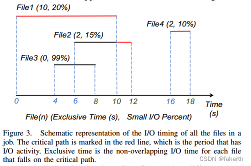
processes in one job produce four files during different time slots. There is also an I/O idle period (between 12 s and 16 s on the x-axis). In this example, the write time reported by Darshan is 18 s; however, the actual write time without the idle time is 14 s. Consequently, this approach downplays the true write bandwidth and can falsely mark a job as a lowperformance instance. Instead, we measure the write time by looking at the timing on the critical path, defined as the period that has I/O activity. In Figure 3, the critical path includes 0 − −12 seconds and 16 − −18 seconds. To find out the critical path, we introduce the concept of critical files, defined as the minimum set of files whose I/O time cover the critical path. In Figure 3, File1, File2, and File4 are the critical files. We further define exclusive time as the non-overlapping portions of I/O time for the critical files.In Figure 3, the exclusive times for File1, File2, and File4 are marked in red, and the lengths are 10 s, 2 s, and 2 s, respectively. The total I/O time is derived by summing up these exclusive times. Following this more accurate timing, we calculate a small I/O percentage of these critical files (Psmall) by Equation 2.

一个作业中的进程在不同的时间段产生四个文件。还有一个I/O空闲时间(在x轴上在12秒到16秒之间)。在本例中，Darshan报告的写时间为18秒;但是，不考虑空闲时间的实际写时间是14秒。因此，这种方法低估了真正的写带宽，并可能错误地将作业标记为低性能实例。相反，我们通过查看关键路径上的时间(定义为有I/O活动的时间段)来测量写入时间。图3中关键路径包括0−−12秒和16−−18秒。为了找出关键路径，我们引入了关键文件的概念，将其定义为I/O时间覆盖关键路径的最小文件集。在图3中，File1、File2和fil4是关键文件。我们进一步将独占时间定义为关键文件的非重叠部分I/O时间。在图3中，File1、File2和fil4的独占时间用红色标记，长度分别为10秒、2秒和2秒。总I/O时间是通过将这些独占时间相加得出的。按照这个更精确的计时，我们通过公式2计算这些关键文件的一个小I/O百分比(Psmall)。

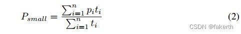
In this equation, pi refers to the small I/O percentage of F ilei , ti refers to the exclusive time of F ilei , and n is the number of critical files. The resultant Psmall is an average of all critical files’ pi weighted by their ratio of exclusive time (ti) to the total I/O time (Pn i=1 ti). The value of nonconsecutive I/O percentage, and OST contention levels can be derived by using the same approach. The benefits of this approach are threefold. First, it helps users precisely filter the low-bandwidth jobs from all the analyzed jobs.Second, it allows users to identify the potential causes for a job’s low performance from the above contributing factor values. Third, for those jobs whose performance does not exhibit strong correlation with the calculated contributing factor values, it provides a list of critical files, so that users can identify the causes from these files’ I/O statistics.

式中，pi表示filei的小I/O百分比，ti表示filei的独占时间，n为关键文件数。由此得到的Psmall是所有关键文件的pi的平均值，其加权值为它们的独占时间(ti)与总I/O时间(Pn I =1 ti)之比。非连续I/O百分比的值和OST争用级别可以通过使用相同的方法得到。这种方法的好处是三重的。首先，它可以帮助用户从所有分析的作业中精确地过滤低带宽作业。其次，它允许用户从上述贡献因素值中确定作业低性能的潜在原因。第三，对于那些性能与计算的贡献因素值没有很强相关性的作业，它提供了一个关键文件列表，以便用户可以从这些文件的I/O统计信息中确定原因。

A key question is how to extract the critical files and their exclusive time. As a naive approach, one can determine the critical files in n rounds of iterations. Each round adds one critical file to the solution by comparing the timing of all the files not in the solution. This approach gives O(n 2 ) complexity. Instead, we solve this problem more efficiently (O(nlog(n))) using a sweep-line algorithm [6]. It is an algorithmic paradigm in computational geometry. The idea behind sweep line is to image a line swept across the whole plane (e.g., the plane containing all the lines in Figure 3), stopping at the points that have I/O activities (e.g., 0, 4, 6, 16 as I/O starts for a file, and 8, 10, 12, 18 as I/O ends), and updating the critical paths and exclusive times upon each activity. The complete solution is available once this line reaches the final activity (e.g., 18 s in Figure 3). The solution is shown in Algorithm 2.

关键问题是如何提取关键文件及其独占时间。作为一种简单的方法，可以在n轮迭代中确定关键文件。通过比较所有不在解决方案中的文件的时间，每轮向解决方案添加一个关键文件。这种方法的复杂度为0 (n2)。相反，我们使用扫描线算法更有效地解决了这个问题(O(nlog(n)))[6]。它是计算几何中的一种算法范例。扫描线背后的思想是在整个平面上扫描一条线(例如，包含图3中所有线的平面)，在有I/O活动的点上停止(例如，文件的I/O开始时为0,4,6,16,I/O结束时为8,10,12,18)，并更新每个活动的关键路径和独占时间。一旦这条线到达最终活动(例如，图3中的18秒)，完整的解决方案就可用了。解决方案显示在算法2中。

Algorithm 2: Sweep-line-based poor I/O analytics
Input: file lst: the list of all the files in a job
Output: share lst: the list of time shares for each file
1 begin
2 	for f in file lst do
3 		points.add((f.start, f.name, type start))
4 		points.add((f.end, f.name, type end))
5 	sort points by time
6 	for p in points do
7 		if p.type == type start then
8 			if heap.size() == 0 then
9 				first = p
10 			heap.push(p)
11 		if p.type == type end then
12 			heap.del(p)
13 			if p.fname == f irst.fname then
14 				share lst.add((first.fname, first.start,p.end))
15 				if heap.size() ! = 0 then
16 					first = heap.peek()
17 					first.start = p.end

Lines 2-4 show an iteration over all the files. Two tuples are created for each file based on its start time and end time, respectively. These points are sorted in an ascending order based on their times (Line 5). Then the algorithm sweeps through all these points (Line 6-17) to add each encountered point of type “start” (referred to as start point) to a heap (Line 10) and to remove it from a heap when its counterpart end point is encountered (Line 12). In doing so, the time range of all stashed points in the heap dynamically changes.

For the scenario shown in Fig. 3, when File1’s start point is added first, the current time range is 0 to 10. When File3’s start point is added next, the range remains as 0 to 10 because File3’s range is 4 to 8, which is a subset of the current range. When File2 is added, the range is adjusted to 0 to 12 based on File2’s range (6 to 12). We can see that the end of the current range varies as new start points are encountered, just like an expanding sweep line. When an end point is encountered (Line 11), its file name is matched with the first start point (first in Line 9) that joins the sweep line (Line 13), if they belong to the same file, this file’s exclusive time is added to the output list (Line 14), and the sweep line is reset by selecting a top point from the heap as the first point of the new sweep line (Line 16), and setting its start time as the current time suggested by p.end (Line 17).

In Fig. 3, File1 ends at 10; it is added to the output list as (File1, 0, 10). At this point, File2 is the only file in the heap (File3 already ends at 8). File2’s entry is selected from the heap and becomes the first of the sweep line. With this algorithm, (File2, 10, 12) and (File4, 16, 18) are added to the output list subsequently.

第2-4行显示了对所有文件的迭代。根据每个文件的开始时间和结束时间分别为其创建两个元组。这些点根据它们的时间按升序排序(第5行)。然后算法遍历所有这些点(第6-17行)，将每个遇到的类型为“start”的点(称为起点)添加到堆中(第10行)，并在遇到对应的终点时将其从堆中删除(第12行)。这样做时，堆中所有存储点的时间范围会动态改变。

对于图3所示的场景，首先添加File1的起始点时，当前时间范围为0到10。当接下来添加File3的起始点时，范围保持为0到10，因为File3的范围是4到8，这是当前范围的一个子集。添加File2时，在File2的取值范围(6 ~ 12)的基础上调整为0 ~ 12。我们可以看到，当前范围的结束随着遇到新的起点而变化，就像扩展的扫描线一样。当一个终点遇到(第11行),它的文件名是与第一个开始点(在第9行),加入扫线(13号线),如果他们属于同一个文件,这个文件的专属时间添加到输出列表(14行),和扫线是重置通过选择一个顶级点从堆中作为第一个点的新扫描行(16行),并设置其开始时间为当前时间p.end提出的(17行)。

在图3中，File1结束于10;它以(File1, 0,10)的形式添加到输出列表中。此时，File2是堆中唯一的文件(File3已经在8处结束)。File2的条目从堆中选择并成为扫描行的第一个。使用此算法，(File2, 10,12)和(fil4, 16,18)随后被添加到输出列表中。

III. EVALUATION

In this section, we evaluate IOMiner’s support for various types of analysis. We ran a large number of analysis tasks, but because of the page limit we present only a few interesting results. We use IOMiner to perform simple analysis tasks that can be accomplished by grouping, sorting, filtering, and projection operations, and in-depth analysis that can be answered by grouping/binning with the userdefined functions. We also discuss our use of IOMiner to find root causes of an application’s poor I/O performance.

在本节中，我们将评估IOMiner对各种类型分析的支持。我们运行了大量的分析任务，但由于页面限制，我们只展示了一些有趣的结果。我们使用IOMiner来执行简单的分析任务，这些任务可以通过分组、排序、过滤和投影操作来完成，而深度分析可以通过使用用户定义的函数进行分组/分组来完成。我们还讨论了使用IOMiner查找应用程序I/O性能差的根本原因。

A. Experimental Setup

We ran IOMiner on the Cray XC40 system Cori at the National Energy Research Scientific Computing Center (NERSC) to analyze the I/O performance logs collected on the same system. Cori consists of two partitions: one has ≈2,400 nodes with Intel Xeon “Haswell” processors, and another has ≈9,700 Intel Xeon Phi “Knights Landing” (KNL) processors. Cori has several different user-accessible file systems, including a disk-based Lustre system, an SSDbased burst buffer, and a disk-based GPFS file system.

我们在国家能源研究科学计算中心(NERSC)的Cray XC40系统Cori上运行IOMiner，以分析在同一系统上收集的I/O性能日志。Cori由两个分区组成:一个分区拥有≈2,400个带有英特尔至强“Haswell”处理器的节点，另一个分区拥有≈9,700个英特尔至强Phi“骑士登陆”(KNL)处理器。Cori有几个不同的用户可访问文件系统，包括基于磁盘的Lustre系统、基于ssd的突发缓冲区和基于磁盘的GPFS文件系统。

B. Performance of IOMiner

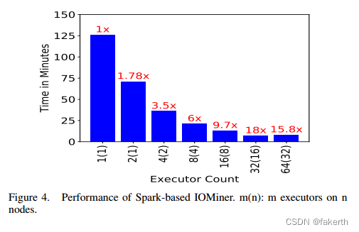
In our first experiment, we demonstrate the execution time of IOMiner in retrieving results to answer “How many jobs use customized stripe configuration?” To answer this question, IOMiner selects all the jobs using Lustre and scans across all the files in each job to determine whether their stripe size, stripe count, and stripe offset are the same as the Lustre’s default setting (1048576, 1, and −1, respectively, for the three parameters).

在我们的第一个实验中，我们演示了IOMiner在检索结果以回答“有多少作业使用自定义条带配置”时的执行时间。为了回答这个问题，IOMiner选择所有使用Lustre的作业，并扫描每个作业中的所有文件，以确定它们的条带大小、条带计数和条带偏移量是否与Lustre的默认设置相同(这三个参数分别为1048576、1和- 1)。

Figure 4 shows IOMiner’s execution times with a varying executor count. We place two executors on each node to leverage its NUMA architecture. We observe that IOMiner performs the best with 32 executors, with 18× speedup over the single-executor case. We also note that increasing executors beyond 32 does not scale, mainly because the data size per executor becomes smaller and communication overhead between the driver and the executors becomes a dominant factor. We have also measured the performance of extracting data directly from Darshan’s own log format using one process, answering this query involves opening, closing and scanning each log for the stripe information, which could not finish in our requested wall time limit (6 hours).

图4显示了不同执行器计数下IOMiner的执行时间。我们在每个节点上放置两个执行器，以利用其NUMA体系结构。我们观察到，IOMiner在使用32个执行器时性能最好，比单执行器的情况提高了18倍。我们还注意到，将执行程序增加到32个以上是不可伸缩的，主要是因为每个执行程序的数据大小变得更小，并且驱动程序和执行程序之间的通信开销成为主要因素。我们还测量了使用一个进程直接从Darshan自己的日志格式提取数据的性能，回答这个查询涉及打开、关闭和扫描每个日志以获取条带信息，这无法在我们要求的墙时间限制(6小时)内完成。

C. First-Order statistics

The results suggest that only 0.08% of jobs adopt a customized stripe setting. This observation raises a concern for those common I/O workloads (i.e., N-1 and N-M in Section III-D) that involve multiple processes concurrently writing/reading the shared files. With a default stripe count of 1, all processes sharing the same file are bottlenecked by the bandwidth of a single OST. Despite this, other HPC centers have reported low rates of custom stripe settings [9].

We performed a set of first-order statistical analyses to provide examples of IOMiner’s capabilities. We discuss new observations in I/O analysis using these analytics.

结果表明，只有0.08%的作业采用了自定义分条设置。这一观察结果引起了对那些涉及多个进程并发地写/读共享文件的常见I/O工作负载(即第III-D节中的N-1和N-M)的关注。默认分条数为1时，共享同一文件的所有进程都会受到单个OST带宽的瓶颈。尽管如此，其他HPC中心报告了较低的自定义条带设置率[9]。

我们执行了一组一阶统计分析，以提供IOMiner功能的示例。我们将使用这些分析讨论I/O分析中的新观察结果。

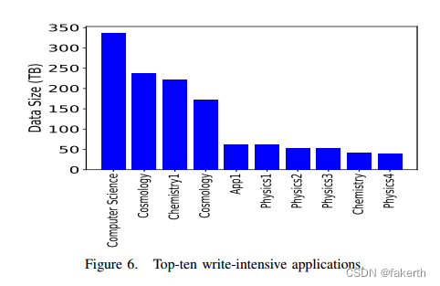
1. Top I/O-intensive applications: The top I/O-intensive applications are of particular interest to the I/O specialists in optimizing applications’ I/O performance and to file system designers in dealing with peak application I/O workloads.We leverage IOMiner to select the top most read- and write-intensive applications by grouping these jobs based on executable names of applications and then calculating the aggregate read/write sizes for all jobs in each application and ranking them by their aggregate bytes read/written. Figures 5 and 6 show the applications and their aggregate read/write sizes. We have anonymized the applications using their science area. Overall, these top ten I/O-intensive applications consume 72% and 76% of the entire read and write traffic captured by Darshan, respectively.

1)顶级I/O密集型应用程序:顶级I/O密集型应用程序对优化应用程序I/O性能的I/O专家和处理峰值应用程序I/O工作负载的文件系统设计人员特别感兴趣。我们利用IOMiner根据应用程序的可执行文件名对这些作业进行分组，然后计算每个应用程序中所有作业的总的读/写大小，并根据其总的读/写字节对它们进行排序，从而选择读写密集程度最高的应用程序。图5和图6显示了应用程序及其总的读/写大小。我们对使用其科学领域的应用程序进行了匿名处理。总的来说，这十大I/ o密集型应用程序分别消耗了Darshan捕获的整个读写流量的72%和76%。

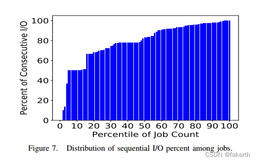
2. Distribution of sequential I/O: Sequential I/O is a friendly I/O pattern for the disk-based file systems and the SSD-based burst buffers. In this pattern, an I/O request issued by a process immediately accesses the end byte of the previous I/O operation. I/O bandwidth can be enhanced by aggregating multiple consecutive writes/reads, which may be smaller than a file system page size, into fewer accesses. To analyze how many HPC applications can benefit from such optimization, we define the ratio of sequential I/O Pseq as Equation 3, where Nseq and Ntot refer to the number of sequential I/O requests and the total reads/writes count in each job. We then calculate the percentile of Pseq and plot its cumulative distribution, as shown in Figure 7. In this figure, each point on the x-axis represents the percentile of jobs whose Pseq is below its value on the y-axis. We can see that only close to 10% of jobs’ Pseq are below 50%; in other words, 90% of jobs’ Pseq are above 50%. In addition, we see that almost half of the jobs’ Pseq are above 80%. This observation implies that sequential I/O is highly prevalent in the HPC I/O workloads and that further I/O optimizations such as I/O aggregation can improve I/O performance.

2)顺序I/O的分布:对于基于磁盘的文件系统和基于ssd的突发缓冲区来说，顺序I/O是一种友好的I/O模式。在这种模式中，进程发出的I/O请求立即访问前一个I/O操作的结束字节。I/O带宽可以通过聚合多个连续的写/读(可能小于文件系统页面大小)到更少的访问来增强。为了分析有多少HPC应用程序可以从这种优化中受益，我们将顺序I/O Pseq的比率定义为公式3，其中Nseq和Ntot指的是顺序I/O请求的数量和每个作业中的总读/写计数。然后我们计算Pseq的百分位数并绘制其累积分布，如图7所示。在该图中，x轴上的每个点表示Pseq低于y轴值的作业的百分位数。我们可以看到，只有近10%的工作的Pseq低于50%;换句话说，90%的工作的Pseq都在50%以上。此外，我们看到几乎一半的工作的Pseq都在80%以上。这一观察结果表明，顺序I/O在HPC I/O工作负载中非常普遍，进一步的I/O优化(如I/O聚合)可以提高I/O性能。

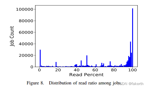
3) Distribution of the read ratio: Checkpointing has been considered as a dominating I/O workload on HPC systems [10], [11], [12], [13]. For this reason, the majority of I/O optimization efforts focus on accelerating checkpointing, a workload featured by bursty writes. In contrast, read optimization has received relatively less attention. However, it remains unknown whether read optimization deserves more effort. To answer this question, we define the read ratio as Equation 4, where Bread and Bwrite refer to the total bytes read and written by each job, respectively. We then bin the jobs based on their Pread into 100 percentiles, and we calculate the job counts in each bin. As can be seen from Figure 8, although a substantial fraction of jobs is either write-only (7% with Pread = 0) or read-only (23% with Pread = 100), the majority of jobs are featured with a mixed workload. In addition, there is a burst of jobs with Pread > 90%, accounting for 53% of the total job count. This analysis informs us that further studies and optimizations on read are worth the investment.

3)读比率的分布:检查点被认为是HPC系统上主要的I/O工作负载[10]，[11]，[12]，[13]。由于这个原因，大多数I/O优化工作都集中在加速检查点上，这是一种以突发写入为特征的工作负载。相比之下，读优化受到的关注相对较少。然而，读优化是否值得更多的努力仍然是未知的。为了回答这个问题，我们将读取比率定义为公式4，其中Bread和Bwrite分别表示每个作业读取和写入的总字节数。然后，我们根据作业的Pread将作业分成100个百分位数，并计算每个分组中的作业数。从图8中可以看出，尽管相当一部分作业要么是只写(Pread = 0时为7%)，要么是只读(Pread = 100时为23%)，但大多数作业的特点是混合工作负载。此外，Pread > 90%的工作岗位激增，占总工作岗位的53%。这个分析告诉我们，对read进行进一步的研究和优化是值得投资的。

D. I/O pattern analysis

N-N and N-1 are considered as two primary I/O patterns of HPC parallel applications [14]. In the N-N pattern, each process (typically, an MPI process) writes/reads a private file. In the N-1 pattern, all the processes concurrently access the same shared file. Many widely adopted I/O benchmarks have been designed to emulate these I/O patterns [15], [16].However, the distribution of I/O pattern usage in parallel applications running on the production HPC systems is an open question. To answer this, we define the file-sharing ratio ® in Equation 5, where P is the process count in a job and F is file count in the job. We use IOMiner to provide a histogram of the job counts based on R, as shown in Figure 9. Note that in the Figure, N-1 case includes the scenario when a list of shared files is accessed by a job, each read/written by all the processes within a distinct time step. We have also excluded the jobs using only one process, which belong to both N-1 and N-N patterns

N-N和N-1被认为是HPC并行应用的两种主要I/O模式[14]。在N-N模式中，每个进程(通常是MPI进程)写/读一个私有文件。在N-1模式中，所有进程并发地访问同一个共享文件。许多广泛采用的I/O基准被设计为模拟这些I/O模式[15]，[16]。然而，运行在生产HPC系统上的并行应用程序中的I/O模式使用分布是一个悬而未决的问题。为了回答这个问题，我们在公式5中定义文件共享比率®，其中P是作业中的进程数，F是作业中的文件数。我们使用IOMiner提供基于R的作业计数的直方图，如图9所示。注意，在图N-1中，用例包括作业访问共享文件列表的场景，每个文件由所有进程在不同的时间步内读/写。我们还排除了只使用一个进程的作业，这些作业属于N-1和N-N模式

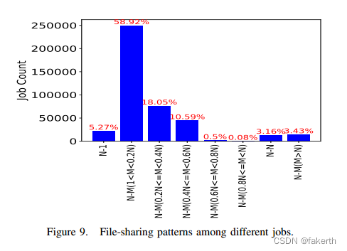
We can see that N-N and N-1 jobs constitute only a small percentage of all the jobs. In contrast, most jobs exhibit the N-M pattern, where either each file is shared by a subset of processes (1 < M < N) or one process works on multiple files (M > N). This observation suggests that existing benchmarks can be adapted to a wider spectrum of file-sharing patterns to more accurately capture the real I/O behavior of the application.

我们可以看到N-N和N-1个作业只占所有作业的一小部分。相比之下，大多数作业都采用N-M模式，其中每个文件由进程子集共享(1 < M < N)，或者一个进程处理多个文件(M > N)。这一观察结果表明，现有基准可以适应更广泛的文件共享模式，以更准确地捕捉应用程序的真实I/O行为。

E. I/O middleware usage analysis

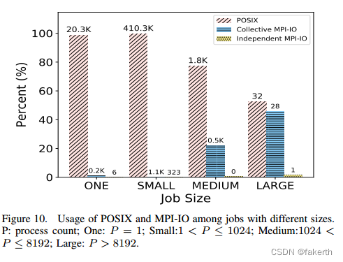
POSIX-IO and MPI-IO have been predominant I/O middleware used for performing parallel I/O. MPI-IO [17] has been developed for roughly two decades to optimize I/O in MPI applications. Its collective I/O optimization, where a small set of MPI processes act as aggregators for performing larger I/O requests to improve performance, is a key optimization method. High-level I/O libraries, such as HDF5 [18] and PnetCDF [19], [20], are built on top of MPIIO to take advantage of various optimizations. While these libraries are efficient for enhancing applications’ I/O performance, it remains unknown how many applications actually use them in production. In this study, we use IOMiner to bin the jobs based on process count, and we calculate the job count using POSIX I/O, MPI-IO in independent mode, and MPI-IO with collective optimizations.

POSIX-IO和MPI-IO一直是用于执行并行I/O的主要I/O中间件。MPI- io[17]已经发展了大约二十年，用于优化MPI应用中的I/O。它的集体I/O优化是一种关键的优化方法，其中一小组MPI进程充当执行较大I/O请求的聚合器，以提高性能。高级I/O库，如HDF5[18]和PnetCDF[19]，[20]，建立在MPIIO之上，以利用各种优化。虽然这些库对于提高应用程序的I/O性能非常有效，但在生产环境中实际使用它们的应用程序的数量仍然未知。在本研究中，我们使用IOMiner根据进程数对作业进行分类，并使用POSIX I/O、独立模式下的MPI-IO和具有集体优化的MPI-IO来计算作业数。

We group four types of jobs based on the process count: MPI jobs using one process (denoted as One); using 2 to 1,024 processes (Small); using 1,025 to 8192 processes (Medium); and using more than 8,192 processes (Large). As shown in Figure 10, among the Darshan logs we evaluated, POSIX I/O is used by 98.8% and 99.6% by single-process (One) and Small jobs, respectively. Although there is a higher use of MPI-IO usage in Medium (22.2%) and Large (45.9%) jobs compared with Small jobs, POSIX-IO remains as the most-used I/O interface. Collective I/O optimizations are enabled in most of the MPI-IO jobs. This situation is probably because of the use of HDF5, the most common parallel I/O library used by the applications on Cori, where collective I/O is enabled. Overall, we can see that although MPI-IO has been a long-standing interface, most HPC users are still committed to POSIX I/O. As I/O specialists spend more effort on the future I/O stacks for exascale computing, one of the challenges is to persuade POSIX-IO users to use the new I/O techniques.

我们根据进程数将四种类型的作业分组:使用一个进程的MPI作业(记为one);使用2到1,024个过程(小);使用1,025到8192个进程(中等);使用超过8192个进程(大型)。如图10所示，在我们评估的Darshan日志中，单进程(One)和Small作业分别使用了98.8%和99.6%的POSIX I/O。虽然与Small作业相比，Medium作业(22.2%)和Large作业(45.9%)的MPI-IO使用率更高，但POSIX-IO仍然是使用最多的I/O接口。在大多数MPI-IO作业中启用了集体I/O优化。这种情况可能是因为HDF5的使用，这是Cori上应用程序使用的最常见的并行I/O库，其中启用了集体I/O。总的来说，我们可以看到，尽管MPI-IO是一个长期存在的接口，但大多数HPC用户仍然致力于POSIX I/O。随着I/O专家在未来用于百亿亿级计算的I/O堆栈上投入更多精力，其中一个挑战是说服POSIX-IO用户使用新的I/O技术。

F. Root Cause Analysis of the Low I/O bandwidth Jobs

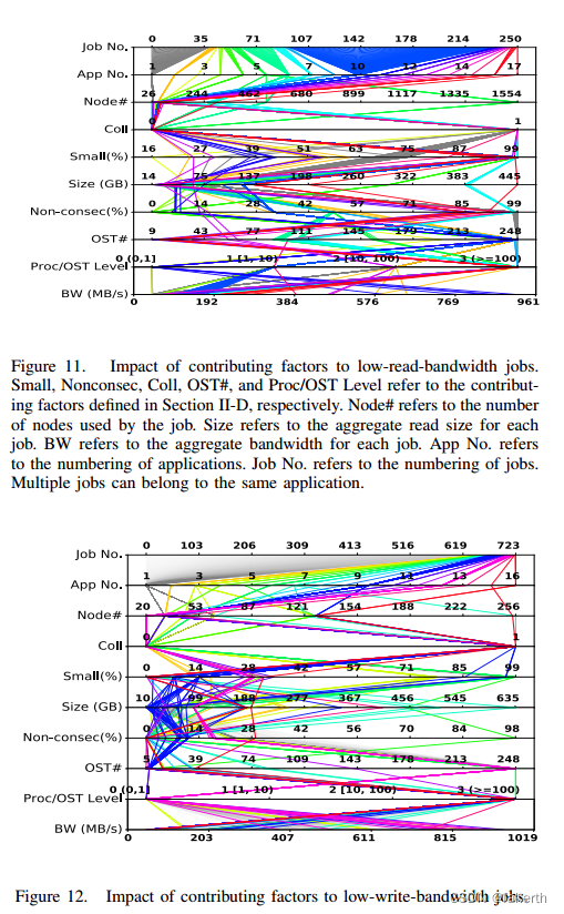
While data-intensive applications running at large scale often can obtain good I/O performance, factors such as I/O pattern, number of I/O requests, and number of storage targets used can affect the sustained performance. To identify the root causes of applications’ low I/O performance, we have used IOMiner in analyzing the logs of jobs using more than 1,000 processes, where each process was writing/reading at least 10 MB of data, and the aggregate sustained I/O bandwidth was lower than 1 GB/s. We then analyzed the root causes of these jobs’ poor I/O bandwidth using the techniques described in Section II-D. The filtering condition returns records pertaining to 251 low-read-bandwidth jobs from 17 applications and to 724 low-write-bandwidth jobs from 16 applications. We show these applications and values of various factors contributing to the I/O performance as parallel coordinate plots [21] in Figures 11 and 12. In these figures, different colors represent different applications. For instance, in Figure 11, we can see that 140 out of 251 jobs are in blue, and they belong to application 10. Since the bandwidth of a job may also be limited by the use of a single node, and the node count information for each job is recorded in a Slurm scheduler log, we also extract this information by joining the Slurm table with the Darshan table (shown as Node#). We found that many jobs experience a contention level (Proc/OST) larger than 3 (e.g. 56 jobs for read, and 395 jobs for write). Further investigation of the I/O logs of these applications revealed their use of default Lustre stripe setting of one OST, causing many processes to concurrently write/read a shared file using the OST, with a resulting bottleneck of the bandwidth on this OST. On the other hand, the impact of collective, small, nonconsecutive I/O and OST count is less perceivable since their values are randomly distributed across their x-axis.

We have also analyzed the well-performing jobs whose bandwidth is beyond 20 GB/s (not shown due to the space limit) and were not able to discover a regular trend among those contributing factors either. These observations inform us that the root causes for jobs’ low I/O performance can be a synergistic effect of multiple contributing factors and thus warrant further analysis of application I/O logs.

虽然大规模运行的数据密集型应用程序通常可以获得良好的I/O性能，但I/O模式、I/O请求数量和所使用的存储目标数量等因素可能会影响持续性能。为了确定应用程序I/O性能低的根本原因，我们使用IOMiner分析了使用1000多个进程的作业的日志，其中每个进程写入/读取至少10 MB的数据，并且总的持续I/O带宽低于1 GB/s。然后，我们使用第II-D节中描述的技术分析了这些作业I/O带宽差的根本原因。过滤条件返回17个应用的251个低读带宽作业和16个应用的724个低写带宽作业的记录。我们在图11和图12中以平行坐标图[21]的形式展示了这些应用程序和影响I/O性能的各种因素的值。在这些图中，不同的颜色代表不同的应用。例如，在图11中，我们可以看到251个作业中有140个是蓝色的，它们属于应用程序10。由于作业的带宽也可能受到单个节点使用的限制，并且每个作业的节点计数信息记录在Slurm调度器日志中，因此我们还通过将Slurm表与Darshan表(如node#所示)连接来提取此信息。我们发现许多作业的争用级别(Proc/OST)大于3(例如56个作业用于读，395个作业用于写)。对这些应用程序的I/O日志的进一步调查显示，它们使用一个OST的默认Lustre stripe设置，导致许多进程使用OST并发地写/读一个共享文件，从而导致该OST上的带宽瓶颈。另一方面，集体的、小的、非连续的I/O和OST计数的影响不太明显，因为它们的值是随机分布在x轴上的。

我们还分析了带宽超过20 GB/s的性能良好的作业(由于空间限制没有显示)，并且也无法发现这些影响因素之间的规律趋势。这些观察结果告诉我们，作业I/O性能低的根本原因可能是多种促成因素的协同效应，因此有必要进一步分析应用程序I/O日志。

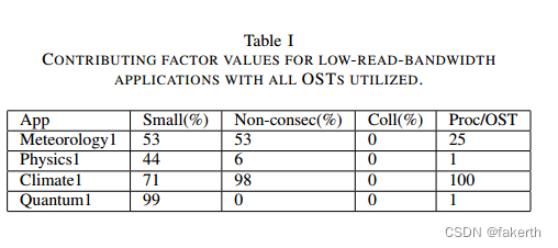
To further investigate the root causes for the individual applications, we select the low-bandwidth jobs that use all the system’s OSTs (248), and we classify them based on their applications. Tables I and II list the contributing values for the low-read-bandwidth and low-write-bandwidth applications, respectively. One can see that jobs belonging to the same applications (same color) generally share similar contributing factor values, so we present the contributing factors of one representative job for each application. The only exception is Physics1 in Table II, where all these jobs share two different sets of contributing factor values (Physics1.1 and Physics1.2).

为了进一步研究单个应用程序的根本原因，我们选择使用所有系统ost(248)的低带宽作业，并根据它们的应用程序对它们进行分类。表1和表2分别列出了低读带宽和低写带宽应用程序的贡献值。可以看到，属于相同应用程序(相同颜色)的工作通常具有相似的贡献因子值，因此我们为每个应用程序提供一个代表性工作的贡献因子。唯一的例外是表II中的Physics1，其中所有这些作业共享两组不同的贡献因子值(Physics1.1和Physics1.2)。

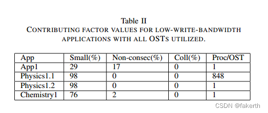
In Table II, we find that the small-write-percentage of Physics1.1, Physics1.2, and Chemistry1 all stay at high values (> 50%). However, we cannot conclude that small writes are the culprit; their writes are mostly consecutive. These small and consecutive writes give the operating system ample opportunity to aggregate the small writes into larger ones. To more precisely find out the causes, we used a sweep-line algorithm (shown in Algorithm 2) to analyze the timing of writing individual files on the critical path. It turns out that the root reason for low performance of Physics1.1 is that its I/O time is bottlenecked by all processes (1,024) writing to one large file on only one OST. The low performance of Physics1.2 and that of Chemistry1 is because the root process writes significantly more data than do the other MPI processes, dominating the write time on critical path. On the other hand, we have also observed that all these contributing factors stay low for App1. Using Algorithm 2, we find that the long I/O time of App1 is because of files being written intermittently and their write times are not well overlapped with each other.
Synchronization also may occur between writing different files, contributing to poor I/O performance.

在表II中，我们发现Physics1.1、Physics1.2和Chemistry1的小写百分比都保持在较高的值(> 50%)。然而，我们不能断定小的写入是罪魁祸首;它们的写入大部分是连续的。这些小而连续的写操作给了操作系统足够的机会将小的写操作聚合成大的写操作。为了更精确地找出原因，我们使用了一种扫描线算法(见算法2)来分析在关键路径上写入单个文件的时间。事实证明，Physics1.1性能低下的根本原因是它的I/O时间被所有进程(1024)只在一个OST上写一个大文件所阻塞。Physics1.2和Chemistry1的低性能是因为根进程比其他MPI进程写更多的数据，控制了关键路径上的写时间。另一方面，我们还观察到，所有这些因素对App1的影响都很低。使用算法2，我们发现App1的I/O时间长是由于文件的写入是间歇性的，并且它们的写入时间没有很好地重叠。在写入不同文件之间也可能发生同步，从而导致较差的I/O性能。

In Table I, we see that the read bandwidths of Meteorology, Climate1, and Quantum1 are impacted by one or multiple factors. For instance, we observe a large percentage of small and nonconsecutive I/O in Meteorology1 and Climate1 (> 50%), which is the primary reason for the two applications’ low read bandwidth.However, we also find that Physics1 is an exception, where all the factors stay at low values. Using Algorithm 2, we observe that reading one file takes up 95% of the total read time on the critical path. These types of root causes could provide sufficient evidence to system administrators at supercomputing facilities for communicating with the users and application developers.

在表1中，我们看到Meteorology, Climate1和Quantum1的读取带宽受到一个或多个因素的影响。例如，我们观察到在Meteorology1和Climate1中有很大比例的小且非连续I/O(> 50%)，这是这两个应用程序的低读带宽的主要原因。然而，我们也发现物理学1是一个例外，所有的因素都保持在低值。使用算法2，我们观察到读取一个文件占用了关键路径上总读取时间的95%。这些类型的根本原因可以为超级计算设施的系统管理员与用户和应用程序开发人员进行通信提供足够的证据。

G. Discussion

Our analysis of the I/O logs on the Cori system at NERSC using IOMiner provides multiple insights. First, read/write traffic on HPC is dominated by only a few applications (Section III-C1), and most applications predominately use sequential I/O (Section III-C2). File system and middleware developers can pay special attention to these top dataintensive applications’ I/O demands and be open to the techniques that boost the sequential I/O bandwidth, such as I/O aggregation. Second, we have identified several directions that are worth further investigation. For instance, read workloads are as common as write workloads (Section III-C3); and optimizations on applications’ read performance, such as data reorganization and caching, can bring significant benefits. POSIX I/O is still the most widely used I/O middleware (Section III-E); hence next-generation I/O stack designs must take into consideration whether POSIX consistency is a real requirement. Since N-M pattern is the most common file-sharing pattern on HPC systems (Section III-D), benchmarks have to be developed to represent this pattern. Furthermore, our root-cause analysis suggests that the reasons for applications’ poor I/O performance can be diverse, either as a result of the synergistic effects of the contributing factors discussed in Section II-D or other factors beyond this scope. With the help of the sweep-line algorithm, HPC users can locate one or multiple bottleneck files on the critical path and find out the root causes for poorI/O-performance by looking only at these files’ statistics.IOMiner provides an extensible and flexible framework to filter a massive number of logs as well as to sift through individual application traces.

我们使用IOMiner对NERSC Cori系统上的I/O日志进行了分析，提供了多种见解。首先，HPC上的读/写流量仅由少数应用程序控制(Section III-C1)，大多数应用程序主要使用顺序I/O (Section III-C2)。文件系统和中间件开发人员可以特别关注这些顶级数据密集型应用程序的I/O需求，并对提高顺序I/O带宽的技术(例如I/O聚合)持开放态度。第二，我们确定了几个值得进一步研究的方向。例如，读工作负载和写工作负载一样普遍(章节III-C3);对应用程序的读性能进行优化，比如数据重组和缓存，可以带来显著的好处。POSIX I/O仍然是使用最广泛的I/O中间件(章节III-E);因此，下一代I/O堆栈设计必须考虑POSIX一致性是否是一个真正的需求。由于N-M模式是HPC系统上最常见的文件共享模式(第III-D节)，因此必须开发基准来表示这种模式。此外，我们的根本原因分析表明，应用程序I/O性能差的原因可能多种多样，可能是第II-D节中讨论的促成因素的协同效应的结果，也可能是超出此范围的其他因素的结果。在扫描线算法的帮助下，HPC用户可以定位关键路径上的一个或多个瓶颈文件，并通过查看这些文件的统计信息找出导致i / o性能低下的根本原因。IOMiner提供了一个可扩展且灵活的框架，用于过滤大量日志以及筛选单个应用程序跟踪。

IV. RELATED WORK

Tracing I/O activity and analyzing the traces has been one of the most prominent techniques for characterizing I/O performance. A limitation of the existing I/O tracing and their performance tools is that the analysis of the traces and statistics and the identification of any performance problems have to be performed manually. Such efforts require expertise in parallel I/O systems. Luu et al [5] have analyzed a large number of Darshan logs collected at multiple supercomputing facilities and summarized that most applications obtain significantly lower I/O performance than the peak capability, and that several applications do not even use parallel I/O libraries. Besides these work on applicationlevel analysis [22], [23], [24], there are numerous work on file system level characterization [25], [26], [27], [28], [29], [30]. These efforts were generally performed manually, and focus on a single level I/O traces, conducting a similar analysis would require significant effort.

跟踪I/O活动并分析跟踪是描述I/O性能的最重要的技术之一。现有I/O跟踪及其性能工具的一个限制是，必须手动执行跟踪和统计分析以及任何性能问题的识别。这样的工作需要并行I/O系统方面的专业知识。Luu等[5]分析了在多个超级计算设施上收集的大量Darshan日志，总结出大多数应用程序的I/O性能明显低于峰值能力，有些应用程序甚至不使用并行I/O库。除了这些关于应用级分析的工作[22]、[23]、[24]，还有大量关于文件系统级表征的工作[25]、[26]、[27]、[28]、[29]、[30]。这些工作通常是手动执行的，并且专注于单个级别的I/O跟踪，执行类似的分析将需要大量的工作。

pytokio [31] is software facilitating holistic characterization and analysis of multi-level I/O traces. It defines abstract connectors to various monitoring tools, and allows users to extract data from these sources using these connectors.Though both pytokio and IOMiner support analytics on multi-level I/O traces, IOMiner differs in that it is designed for large-scale parallel analytics. GUIDE [32] is another framework for analyzing multi-level I/O traces, different from GUIDE, IOMiner focuses more on applications’ I/O behavior and their performance impact, which is useful for both the facility operators and the application developers, while GUIDE targets to deliver system-level statistics to the facility operators, such as the file system workload, the network traffic, etc.

pytokio[31]是一款软件，可以对多级I/O迹线进行整体表征和分析。它定义了到各种监视工具的抽象连接器，并允许用户使用这些连接器从这些源提取数据。尽管pytokio和IOMiner都支持对多级I/O跟踪进行分析，但IOMiner的不同之处在于它是为大规模并行分析而设计的。GUIDE[32]是另一个用于分析多级I/O轨迹的框架，与GUIDE不同，IOMiner更关注应用程序的I/O行为及其对性能的影响，这对设施运营商和应用程序开发人员都很有用，而GUIDE的目标是向设施运营商提供系统级统计数据，如文件系统工作负载、网络流量等。

V. CONCLUSIONS AND FUTURE WORK

In this paper, we present a holistic I/O analysis framework called IOMiner. IOMiner provides unified interfaces and read-friendly storage schema for users to perform an integrated analysis on different types of instrumentation data, such as application and file-system-level logs and job scheduler logs. The whole framework is built on top of Spark and is optimized for parallel queries of HPC storage.Furthermore, IOMiner allows users to conveniently identify the root causes for an application’s poor I/O performance based on a sweep-line algorithm. Our analysis provides several novel insights for HPC users and demonstrates that the root causes for an application’s low I/O performance can be diverse. As future work, we will extend IOMiner with the ability to intelligently learn the new contributing factors for low I/O performance, identify the list of contributing factors that synergistically account for the low performance, and perform system-wide application I/O diagnostics. We will also provide support for more types of I/O instrumentation data under our framework. For instance, ggiostat [33] is a monitoring tool for the GPFS [34] file system. It could be integrated into IOMiner framework in the same way as LMT.

在本文中，我们提出了一个名为IOMiner的整体I/O分析框架。IOMiner为用户提供了统一的接口和易于阅读的存储模式，以便对不同类型的检测数据(如应用程序和文件系统级日志以及作业调度器日志)执行集成分析。整个框架建立在Spark之上，并针对HPC存储的并行查询进行了优化。此外，IOMiner允许用户基于扫描线算法方便地识别应用程序I/O性能差的根本原因。我们的分析为HPC用户提供了一些新颖的见解，并证明了应用程序低I/O性能的根本原因可能是多种多样的。在未来的工作中，我们将扩展IOMiner，使其能够智能地学习导致低I/O性能的新因素，识别协同导致低性能的因素列表，并执行系统范围的应用程序I/O诊断。我们还将在我们的框架下为更多类型的I/O检测数据提供支持。例如，ggiostat[33]是GPFS[34]文件系统的监视工具。它可以像LMT一样集成到IOMiner框架中。