cs224w-图机器学习-Colab 3-GCN在pytorch-geometric中的实现

最新推荐文章于 2022-11-17 20:07:11 发布

知之之

最新推荐文章于 2022-11-17 20:07:11 发布

阅读量317

点赞数

分类专栏： Graph cs224w 文章标签： pytorch

本文链接：https://blog.csdn.net/weixin_43963453/article/details/119966615

版权

cs224w 同时被 2 个专栏收录

14 篇文章 2 订阅

订阅专栏

Graph

13 篇文章 1 订阅

订阅专栏

GCN在pytorch-geometric中的实现

1.图数据卷积范式
2.实现消息传播的三个部分
3.GCN的实现
4. Edge Convolution实现
5.torch_scatter.scatter()解释

官方文档是这里：MESSAGE PASSING NETWORKS

1.图数据卷积范式

文档中说到，Generalizing the convolution operator to irregular domains is typically expressed as a neighborhood aggregation or message passing scheme. 即，在图这种不规则数据上进行卷积运算，都能表示为信息传递模型。 $\mathbf{x}^{(k-1)}_{i}\in\mathbb{R}^{F}$ 为节点 $i$ 在第 $k - 1$ 层的卷积结果表示， $e_{i,j}\in\mathbb{R}^{D}$ 为节点 $j$ 指向节点 $i$ 的边的feature（这是可选的）。那么message passing模型就可以表示为如下的公式： $\mathbf{x}^{(k)}_{i} = \gamma^{(k)}(\mathbf{x}^{(k-1)},\square_{j\in \mathcal{N}(i)}\phi^{(k)}(\mathbf{x}^{(k-1)}_{i},\mathbf{x}^{(k-1)}_{j},\mathbf{e}^{(k-1)}_{i,j}))$
其中在这里插入图片描述
这公式真难打！！

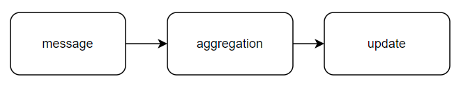
2.实现消息传播的三个部分

如上节的公式所述，这里采用的模型是：
先根据message处理message，然后聚合数据，然后更新表示。这分别对应上述公式中的
$\phi$ , $\square$ , $\gamma$ 。
在这里插入图片描述

（1） $\phi$ ，MessagePassing.message(…)

（2） $\square$ ，aggregation scheme

这个只有三种选择：
“add”, “mean” or “max”

（3） $\gamma$ ，MessagePassing.update(aggr_out, …)

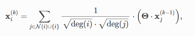
3.GCN的实现

先附上公式。现在任务是根据库中的框架，实现这个操作。只要实现一层的传播就可以了。因此，现在的任务就是根据输入的特征向量 $\mathbf{x}$ ，设定好线性投影的维度后，实现一次传播：
在这里插入图片描述

the forward function is where the actual message passing is conducted. All logic in each iteration happens in forward, where we’ll call propagate function to propagate information from neighbor nodes to central nodes. So the general paradigm will be pre-processing -> propagate -> post-processing.

Recall the process of message passing we introduced in homework 1.
propagate further calls message which transforms information of neighbor nodes into messages, aggregate which aggregates all messages from neighbor nodes into one, and update which further generates the embedding for nodes in the next iteration.

即：在forward函数中做一些预处理，然后调用propagate函数。
propagate函数会自动调用message函数，让它对信息处理。预处理完信息后，调用aggregate 进行聚合。聚合完成后，用update 更新表示。

class GCNConv(MessagePassing):
    def __init__(self, in_channels, out_channels):
        super(GCNConv, self).__init__(aggr='add')  # "Add" aggregation (Step 5).
        self.lin = torch.nn.Linear(in_channels, out_channels)

    def forward(self, x, edge_index):
        # x has shape [N, in_channels]
        # edge_index has shape [2, E]

        # Step 1: Add self-loops to the adjacency matrix.
        edge_index, _ = add_self_loops(edge_index, num_nodes=x.size(0))

        # Step 2: Linearly transform node feature matrix.
        x = self.lin(x)

        # Step 3: Compute normalization.
        row, col = edge_index
        deg = degree(col, x.size(0), dtype=x.dtype)
        deg_inv_sqrt = deg.pow(-0.5)
        deg_inv_sqrt[deg_inv_sqrt == float('inf')] = 0
        norm = deg_inv_sqrt[row] * deg_inv_sqrt[col]

        # Step 4-5: Start propagating messages.
        return self.propagate(edge_index, x=x, norm=norm)

    def message(self, x_j, norm):
        # x_j has shape [E, out_channels]

        # Step 4: Normalize node features.
        return norm.view(-1, 1) * x_j

（1）forward

看下这个函数的实现：

1.修改边矩阵，加上自环

====================================================

 def forward(self, x, edge_index):
        # x has shape [N, in_channels]
        # edge_index has shape [2, E]

        # Step 1: Add self-loops to the adjacency matrix.
        edge_index, _ = add_self_loops(edge_index, num_nodes=x.size(0))

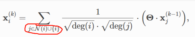
这一步（上面代码中最后一句）对应着公式中，聚合的信息来自邻居+自己（下标那）：
在这里插入图片描述

2.对x线性投影

====================================================

 # Step 2: Linearly transform node feature matrix.
        x = self.lin(x)

这一步是将每个输入的 $\mathbf{x}$ 进行一次线性投影。其中投影层已经定义好了（在__init__()中定义的）。

3.开始计算归一化常数

 # Step 3: Compute normalization.
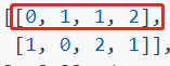
        row, col = edge_index

这一步卡了很久没懂。这edge_index分明是一个Tensor，为什么还能这样给两个值赋值呢？最后debug才发现，edge_index是一个2xEdges的Tensor，
row就是第一行（即头结点，这里假设这是一个有向图。或者说某个边对应的一个节点的index），col就是第二行，即尾结点（即尾结点）。如果是下面的图：
在这里插入图片描述
那么edge_index就是：

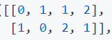
那么row就是红色圈出的那行， col就是下面哪一行。我惊讶于Tensor还能这么赋值。

====================================================

3.计算归一化常数

	deg = degree(col, x.size(0), dtype=x.dtype)
	deg_inv_sqrt = deg.pow(-0.5)
	deg_inv_sqrt[deg_inv_sqrt == float('inf')] = 0
	norm = deg_inv_sqrt[row] * deg_inv_sqrt[col]

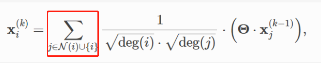
这四句，是为了将所有的边都除以那个归一化因子（下图红色部分）:
在这里插入图片描述
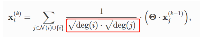
这里实现的逻辑和我想的不一样，所以才会一直不理解。这里归一化数据时，是一次性将所有数据都归一化，而不是先选中节点 $i$ 的邻居，然后做归一化。
这点很关键。
因此，这里先把所有存在的边，对应的归一化因子算出来，然后作为一个参数，供后面使用。
画一下图示意：

在这里插入图片描述
在先算好这几个矩阵后，再讲矩阵传给propagate函数，让它根据index，去找到一个节点的邻居然后聚合。所以关键思想是：先算好一切数据（计算好系数啥的），最后再进行选中、求和操作。

4.准备完成，调用propagate函数更新embedding

====================================================

 # Step 4-5: Start propagating messages.
        return self.propagate(edge_index, x=x, norm=norm)

这一步就是进行消息传递、聚合操作了。文档中这么描述的：

The initial call to start propagating messages. Takes in the edge
indices and all additional data which is needed to construct messages
and to update node embeddings.
即，接受边的信息，和其他需要的数据，进行更新embedding的操作

在这里插入代码片

所有的传播、聚合、信息处理操作，都被这个函数调用。

（2）propagate

这个函数调用了设定好的聚合、message函数等。
这函数中有这句：

	out = self.message(**msg_kwargs)

即调用之前设置好的message()函数。其中的参数是forward函数传来的。
然后一堆看不懂的。下一个关键语句是：

 	out = self.aggregate(out, **aggr_kwargs)

即，调用聚合函数。
最后有句关键的：

	return self.update(out, **update_kwargs)

即调用update函数，更新节点的表示。

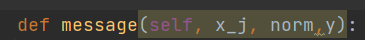
（3）message

这是官网的文档：
在这里插入图片描述
关键有两点。首先是这函数的目的，即对于每个中心节点 $i$ ，构建传播到它的信息。其次是下标。下标_i代表中心节点，_j代表邻居节点。
所有传给propagate()的参数，这函数都能用。不同点就在于加了下标。
上面传给propagate()函数的x，形状是 $37 * 32$ ,即 $37 个节点，每个节点有 32 维的嵌入$ 。但是传给本函数message()的参数是这俩：
在这里插入图片描述
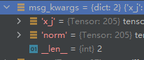
x_j是 $205 * 32$ 的，对应边顺序的节点嵌入。可能是为了方便计算，毕竟这只是将之前 $37 * 32$ 的嵌入重拍复制了一下。norm是 $205 * 1$ 的，对应205个边的归一化因数。
但是这有个问题：x_j这个参数是必须会有的吗？是不需设置，就能得到的吗？源码的实现中就有x_j，看来应该是必有的
：源码链接

def message(self, x_j: Tensor) -> Tensor:
        r"""Constructs messages from node :math:`j` to node :math:`i`
        in analogy to :math:`\phi_{\mathbf{\Theta}}` for each edge in
        :obj:`edge_index`.
        This function can take any argument as input which was initially
        passed to :meth:`propagate`.
        Furthermore, tensors passed to :meth:`propagate` can be mapped to the
        respective nodes :math:`i` and :math:`j` by appending :obj:`_i` or
        :obj:`_j` to the variable name, *.e.g.* :obj:`x_i` and :obj:`x_j`.
        """
        return x_j

为了验证这个问题，我给propagate()函数加了一个参数y，然后也给message()函数加了一个参数y。发现是一个东西：
注释掉的是原来的函数。
在这里插入图片描述
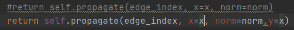
这是给message()函数加了参数y后的：

在这里插入图片描述
这是debug的结果：

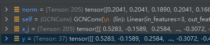
可以看出，message()函数中的y，和propagate()中的，一样。norm参数也一样。

（4）update

这是原本的函数实现：
在这里插入图片描述
可以看出，和message()很像，都是空的。如果不重写的话，就是什么也不做的实现。（看源码真有用，只是太难了）

（5）总结

forward函数先做预处理，然后调用propagate函数。propagate函数会调用message和aggregate函数。所以需要修改啥，就改啥。直接继承MessagePassing这个类，然后重写函数就行。

4. Edge Convolution实现

一鼓作气。学了GCN的实现，文档中还附了 Edge Convolution的实现。这个就很容易理解了：
在这里插入图片描述
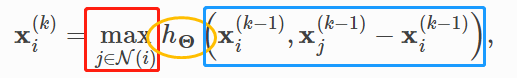
红方框是聚合函数max；橙椭圆是MLP，message函数；蓝方框是预处理。

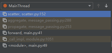
5.torch_scatter.scatter()解释

理解这个函数，是理解上述实现的“手筋”。因为大概了解了这个函数，才知道库中采用的方法是“先算好数据，最后再进行求和啥的操作”。
函数的文档
这函数是被aggregate()函数调用的。
我运行的测试代码如下：

import torch
from torch_geometric.nn import MessagePassing
from torch_geometric.utils import add_self_loops, degree
from torch_geometric.datasets import TUDataset

dataset = TUDataset(root='/tmp/ENZYMES', name='ENZYMES')
data = dataset[0]

class GCNConv(MessagePassing):
    def __init__(self, in_channels, out_channels):
        super(GCNConv, self).__init__(aggr='add')  # "Add" aggregation (Step 5).
        self.lin = torch.nn.Linear(in_channels, out_channels)

    def forward(self, x, edge_index):
        # x has shape [N, in_channels]
        # edge_index has shape [2, E]

        # Step 1: Add self-loops to the adjacency matrix.
        edge_index, _ = add_self_loops(edge_index, num_nodes=x.size(0))

        # Step 2: Linearly transform node feature matrix.
        x = self.lin(x)

        # Step 3: Compute normalization.
        row, col = edge_index
        deg = degree(col, x.size(0), dtype=x.dtype)
        deg_inv_sqrt = deg.pow(-0.5)
        deg_inv_sqrt[deg_inv_sqrt == float('inf')] = 0
        norm = deg_inv_sqrt[row] * deg_inv_sqrt[col]

        # Step 4-5: Start propagating messages.
        return self.propagate(edge_index, x=x, norm=norm)

    def message(self, x_j, norm):
        # x_j has shape [E, out_channels]

        # Step 4: Normalize node features.
        return norm.view(-1, 1) * x_j
conv = GCNConv(3, 32)
x = conv(data.x, data.edge_index)

debug栈帧如下：
在这里插入图片描述
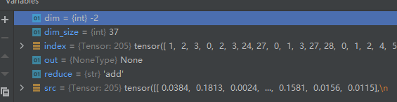
调用这个函数的参数如下：其中inputs是 $205 * 32$ 的特征矩阵。

可以看到，当选用求和函数作为aggregate函数时，函数最终调用的实现是torch_scatter.scatter()。这个函数是这样的：
在这里插入图片描述
可以看到其debug的数据。
这个函数的作用大概是这样：

可以看到，上面的参数是：

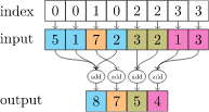
即，按照index（即前面的edge的row参数，红色方框内），对上面input进行求和。如果是下图的数据，则对0的节点求一次和，对1的节点求一次和，对2 的求一次。最后是3个和。但是debug的数据index有 $37$ 个不同的数据（对应37个不同的节点），所以输出也是 $37 * 32$ 的，即输出的是下一层的表示。
在这里插入图片描述
这个scatter函数，比如现在对1这个节点求和，就相当于找到1的所有邻居节点对应的表示，然后求和。对应公式中这部分：

知之之

关注

0
点赞
踩
1

收藏

觉得还不错? 一键收藏
0
评论
cs224w-图机器学习-Colab 3-GCN在pytorch-geometric中的实现

实现记录一、GNN在pytorch-geometric中的实现思路1.实现GNN的思路一、GNN在pytorch-geometric中的实现思路官方文档是这里：MESSAGE PASSING NETWORKS1.实现GNN的思路文档中说到，Generalizing the convolution operator to irregular domains is typically expressed as a neighborhood aggregation or message passing s
复制链接

扫一扫