


PointConv论文阅读笔记
Abstract
本文发表于CVPR。 其主要内容正如标题,是提出了一个对点云进行卷积的Module,称为PointConv。由于点云的无序性和不规则性,因此应用卷积比较困难。
其主要的思路是,将卷积核当做是一个由权值函数和密度函数组成的三维点的局部坐标的非线性函数。通过MLP学习权重函数,然后通过核密度估计得到密度函数。
还有一个主要的贡献在于,使用了一种高效计算的方法,转换了公式的计算分时,使得PointConv的卷积操作变得memory efficient,从而加深网络的深度。
This paper first published on CVPR. In this paper, author proposed a novel convolution operation which can be directly used on point cloud. As we all know, unlike image whose pixels are fixed, point cloud is irregular and unordered. So directly extend convolution operation into 3D pointcloud can be difficult.
Author treat convolution kernels as nonlinear functions of the local coordinates of 3D points comprised of weight function and density function. The wight function is learned by multi-layer perceptron networks, the density function is learned through kernel density estimation.
Another main contribution of their work is that they reformulate the proposed convolution method to make it more memory efficient which significantly improves the depth of the network.
About PointConv
作者提出了一种全新的,考虑到非均匀采样,对三维点云进行卷积的途径。 我们知道,卷积操作可以被看做是连续意义上的卷积函数的离散化近似。 在三维空间中,我们将卷积算子的权重函数视为是在以某个三维点为参考点的局部坐标系下的连续函数。该函数可以使用多层感知机进行模拟。这部分工作在之前已经有人做过,但是全部没有考虑到非均匀采样的问题。
基于这个Motivation,我们进一步使用一个逆密度尺度来对MLP学到的权重函数进行重新计算,对应于原连续卷积函数的蒙特卡罗近似。我们将其称为PointConv。 PointConv以点云的位姿作为输入,通过MLP学习权重函数,然后再应用一个inverse density scale, 对权重函数进行重新计算,以弥补点云数据是由非均匀采样采得所带来的影响。
PointConv最简单的实现是很消耗内存的,当输出通道的维度很大时,会给训练带来很大难度。 为了减少PointConv的内存消耗,作者通过改变加和顺序对公式进行了重写,大大提高了效率。
此外,由于PointConv是卷积操作的完整近似,所以很容易就能从Conv推广到DeConv。DeConv层,也就是反卷积层,能够充分利用从粗糙层得到的信息,并将之传送到精细层去。而之前的很多卷积操作,不是full approxiamtion,所以就无法反卷积。对性能有很大影响。
Author proposed a novel approach to apply convolution operation on 3D point clouds with consideration on non-uniform sampling. Note that convolution operation can be viewed as a discrete approximation of a continuous convolution operator. In 3D space, we can treat the weights of this convolution operator to be a continous function of the local 3D point coordinates with respect to a reference 3D point. The continuous function can be approximated by a multi-layer perceptron(MLP). This work has be done before, but all of them didn’t take non-uniform sampling into consideration.
Based on this motivation, author used an inverse density scale to re-weight the continuous function learned by MLP, which correspond to the Monte Carlo approximation of the continuous convolution. PointConv involves taking the positions of point clouds as input and learning an MLP to approximate a weight function, as well as applying a inverse density scale on learned weights to compensate the non-uniform sampling.
The naive implementation of PointConv is memory inefficient when the channel size of the output features is very large and hence hard to train and scale up to large networks. In order to reduce the memory consumption of PointConv, author introduced an approach which is able to greatly increase the memory efficiency using a reformulation that changes the summation order.
PointConv is full approximation of the convolution, it’s natural to extend PointConv to a PointDeconv, which an fully untilize the information in coarse layer and propagate to finer layers while most state of art algorithm cannot perform deconvolution because they are not the full approximation.
Convolution on 3D Point Clouds
d维向量的卷积定义如下:
(
f
∗
g
)
(
x
)
=
∬
τ
∈
R
d
f
(
τ
)
g
(
x
+
τ
)
d
τ
(f*g)(x) = \iint\limits_{\tau \in {\mathbb{R}^d}} {f(\tau )g(x + \tau )d\tau }
(f∗g)(x)=τ∈Rd∬f(τ)g(x+τ)dτ
二维图像image的像素点是固定的。每个像素点会固定在某个体素网格。而点云不同,一个点云可以被表示为一个三维点集,其中每个点都包含着一个位置向量,同时还有其特征如颜色,表面向量等。不同于图像,点云有着更加灵活的形状,一个点的坐标(x,y,z)不会位于某个确定的网格上,而是可以取一个任意的连续值。因此,局部区域内不同点之间的相对位置是十分多变的。传统的光栅图像离散卷积滤波器不能够直接应用于3D点云上。
为了得到一个能够应用于三维点云的卷积操作,首先回到连续的三维卷积:
C
o
n
v
(
W
,
F
)
x
y
z
=
∭
(
δ
x
,
δ
y
,
δ
z
)
∈
G
W
(
δ
x
,
δ
y
,
δ
z
)
F
(
x
+
δ
x
,
y
+
δ
y
,
z
+
δ
z
)
d
δ
x
δ
y
δ
z
Conv{(W,F)_{xyz}} = \iiint\limits_{({\delta _x},{\delta _y},{\delta _z}) \in G} {W({\delta _x},{\delta _y},{\delta _z})F(x + {\delta _x},y + {\delta _y},z + {\delta _z})d{\delta _x}{\delta _y}{\delta _z}}
Conv(W,F)xyz=(δx,δy,δz)∈G∭W(δx,δy,δz)F(x+δx,y+δy,z+δz)dδxδyδz
其中 F ( x + δ x , y + δ y , z + δ z ) F(x+\delta_x,y+\delta_y,z+\delta_z) F(x+δx,y+δy,z+δz)是以 ( x , y , z ) (x,y,z) (x,y,z)为中心的局部区域 G G G中点的特征。点云可以被看做是从连续空间 R 3 \mathbb{R}^3 R3中非均匀采样得到的。 δ x , δ y , δ z {\delta _x},{\delta _y},{\delta _z} δx,δy,δz是局部区域内的任意位置的三维坐标。
那么PointConv定义如下:
P
o
i
n
t
C
o
n
v
(
S
,
W
,
F
)
x
y
z
=
∑
(
δ
x
,
δ
y
,
δ
z
)
∈
G
S
(
δ
x
,
δ
y
,
δ
z
)
W
(
δ
x
,
δ
y
,
δ
z
)
F
(
x
+
δ
x
,
y
+
δ
y
,
z
+
δ
z
)
PointConv{(S,W,F)_{xyz}} = \sum\limits_{({\delta _x},{\delta _y},{\delta _z}) \in G} {S({\delta _x},{\delta _y},{\delta _z})W({\delta _x},{\delta _y},{\delta _z})F(x + {\delta _x},y + {\delta _y},z + {\delta _z})}
PointConv(S,W,F)xyz=(δx,δy,δz)∈G∑S(δx,δy,δz)W(δx,δy,δz)F(x+δx,y+δy,z+δz)
对连续函数的离散化近似从上可窥一见。 其中
S
(
δ
x
,
δ
y
,
δ
z
)
S({\delta _x},{\delta _y},{\delta _z})
S(δx,δy,δz)是点
(
δ
x
,
δ
y
,
δ
z
)
({\delta _x},{\delta _y},{\delta _z})
(δx,δy,δz)处的逆密度inverse density。由于点云采样的非均匀性,
S
(
δ
x
,
δ
y
,
δ
z
)
S({\delta _x},{\delta _y},{\delta _z})
S(δx,δy,δz)是十分有必要的。直觉上讲,点云内不同局部区域内的点的个数是很不相同的。
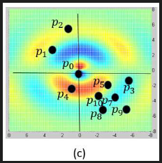
如上图,因为点 p 3 , p 5 , p 6 , p 7 , p 8 , p 9 , p 10 p_3,p_5,p_6,p_7,p_8,p_9,p_{10} p3,p5,p6,p7,p8,p9,p10之间离得都很近,所以它们每一个的贡献度应该更小。inverse density的原因。就是采样密度越大,这里点的人均贡献度应该越小。
PointConv的公式如上。
PointConv的具体实现
我们使用MLP来从三维坐标 ( δ x , δ y , δ z ) ({\delta _x},{\delta _y},{\delta _z}) (δx,δy,δz)中近似得到权重函数 W ( δ x , δ y , δ z ) W({\delta _x},{\delta _y},{\delta _z}) W(δx,δy,δz). 而逆密度函数 S ( δ x , δ y , δ z ) S({\delta _x},{\delta _y},{\delta _z}) S(δx,δy,δz) 则由一个核密度估计及紧随其后的一个由MLP实现的非线性转换实现。
计算权重函数的MLP的参数是在所有点上共享的,以达到扰动不变性的目的。 而逆密度函数首先需要估计点云在某点处的密度(kernel density estimation(KDE)),然后将这个估计出来的密度送入一个MLP来进行一个一维的非线性变换。其目的是在于让网络决定,是否去使用密度估计。

首先得明确上图这个网络的输入和输出。
输入是 F i n F_{in} Fin,shape是 K × C i n K \times C_{in} K×Cin, 也就是说要对某个点进行卷积,那么它的输入是k个邻居的feature(当前维的feature是 C i n C_{in} Cin). 此外输入还有 P l o c a l , D e n s i t y P_{local}, Density Plocal,Density,一个是k近邻的局部坐标, K × 3 {K \times 3} K×3, 一个是k近邻处的密度, K × 1 K \times 1 K×1。
输出是 F o u t F_{out} Fout,shape为 1 × C o u t 1 \times C_{out} 1×Cout。
C i n , C o u t C_{in}, C_{out} Cin,Cout是输入输出feature的通道数。 k , c i n , c o u t k, c_{in}, c_{out} k,cin,cout分别指第 k k k个邻接点,输入feature的第 c i n c_{in} cin个通道, 输出feature的第 c o u t c_{out} cout个通道。
因为每个点的权重函数不同,且其用于将 C i n C_{in} Cin变换到 C o u t C_{out} Cout, 所以weight function的shape应该为 K × ( C i n × C o u t ) K \times (C_{in} \times C_{out}) K×(Cin×Cout), 即 W ∈ R K × ( C i n × C o u t ) W \in \mathbb{R}^{K \times (C_{in} \times C_{out})} W∈RK×(Cin×Cout). 那么第k个点处应用于第 c i n c_{in} cin个通道上的weight function应该是一个向量: W ( k , c i n ) ∈ R C o u t W(k,c_{in}) \in \mathbb{R}^{C_{out}} W(k,cin)∈RCout
所以有:
F
o
u
t
=
∑
k
=
1
K
∑
c
i
n
=
1
C
i
n
S
(
k
)
W
(
k
,
c
i
n
)
F
i
n
(
k
,
c
i
n
)
{F_{out}} = \sum\limits_{k = 1}^K {\sum\limits_{{c_{in}} = 1}^{{C_{in}}} {S(k)W(k,{c_{in}}){F_{in}}(k,{c_{in}})} }
Fout=k=1∑Kcin=1∑CinS(k)W(k,cin)Fin(k,cin)
上图中有tile的操作,相当于人为广播broadcast.
PointConv通过网络学习得到权重函数W的离散化模拟,对于每个输入点,通过MLP使用其相对坐标来计算权重。下图(a)举了一个连续的权重函数用于卷积的例子,而点云是对连续输入(i.e.空间)的离散化处理(i.e.采样),我们通过图(b)类似的方式进行离散化卷积来抽象出局部特征(对于不同的采样会输出不同的W和S,所以其效果也不同)。 需要说明的是,对于光栅图像,其某个局部区域内的相对坐标都是固定的(体素化网格),所以经过PointConv时,对于整个图像,会输出相同的权重函数W和密度函数S,会变为传统的离散卷积。(所以作者还在后文专门进行了实验,将二维图像升维到三维空间中,通过PointConv,结果确实和二维一致。所以证明了PointConv确实是三维连续卷积的full approximation。
PointDeConv
Efficient PointConv
这两个part搁置一下。因为我感觉论文的核心Part就是如何理解三维点云上的卷积操作。核心部分已经记录了。
而且这篇论文我私以为存在一些问题,作者文中提到more details can be found in supplementary materials, 但是在哪都找不到他的补充材料,并且github上公开的源码并没有efficient realization of PointConv. 作者也不回答这些问题。


 3890
3890


 被折叠的 条评论
为什么被折叠?
被折叠的 条评论
为什么被折叠?
 到【灌水乐园】发言


