[数据分析实践]-Image Matching-2DTo3D-1

最新推荐文章于 2023-10-03 13:01:08 发布

浩波的笔记

最新推荐文章于 2023-10-03 13:01:08 发布

阅读量737

点赞数 1

分类专栏：数据分析文章标签：数据分析 3d 计算机视觉

原文链接：https://www.kaggle.com/code/dschettler8845/image-matching-challenge-2022-eda

版权

数据分析专栏收录该内容

14 篇文章 0 订阅

订阅专栏

数据背景

让机器学习使用互联网上免费提供的大量非结构化图像集合，来帮助更好地捕捉世界的丰富性，这个想法怎么样？从图像重建 3D 对象和建筑物的过程称为运动结构 (SfM)。通常，这些图像是由熟练的操作员在受控条件下捕获的，以确保数据的均匀、高质量。考虑到各种各样的视点、照明和天气条件、人和车辆的遮挡，甚至是用户应用的过滤器，从各种图像构建3D模型要困难得多。

问题的第一部分是识别两个图像的哪些部分捕获场景的相同物理点，例如窗口的角落。这通常通过局部特征（图像中可以在不同视图中可靠识别的关键位置）来实现。局部特征包含捕获兴趣点周围外观的简短描述向量，通过比较这些描述符，可以在两个或多个图像的图像位置的像素坐标之间建立可能的对应关系。这种“图像配准”使得通过三角测量恢复点的 D位置成为可能。

数据介绍

数据集来源：https://www.kaggle.com/competitions/image-matching-challenge-2022/data

下载方式：https://github.com/Kaggle/kaggle-api
kaggle competitions download -c image-matching-challenge-2022

train/*/calibration.csv
- image_id:图像文件名
- camera_intrinsics:此图像的3X3 calibration矩阵K, 通过行索引将其展平为向量
- rotation_matrix:此图像的3X3 rotation矩阵R, 通过行索引将其展平为向量
- translation_vector:转移向量
train/*/pair_covisibility.csv:
- pair:标识一对图像的字符，编码为两个图像文件名由连字符分隔（不带扩展名）
- covisibility:估计两个图像之间的重叠,数字越大表示重叠越大。我们建议使用所有具有0.1或更高共可见性估计值的对。
- fundamental_matrix: 源自calibration文件的目标列
train/scaling_factors.csv:通过 Structure-from-Motion 重建的每个场景的姿势，并只能精确到比例因子。该文件包含每个场景的标量，可用于将它们转换为米进制。
train/*/images/:一批图像都是在同一位置附近拍摄的。
train/LICENSE.txt:每个图像的具体来源和许可的记录。
1test.csv1:
- sample_id: 图像对的唯一标识符。
- batch_id: 批次ID。
- image_[1/2]_id:对中每个图像的文件名。

导入函数库 ⤒

print("\n... IMPORTS STARTING ...\n")

print("\n\tVERSION INFORMATION")
# Machine Learning and Data Science Imports
import tensorflow as tf; print(f"\t\t– TENSORFLOW VERSION: {tf.__version__}");
import tensorflow_hub as tfhub; print(f"\t\t– TENSORFLOW HUB VERSION: {tfhub.__version__}");
import tensorflow_addons as tfa; print(f"\t\t– TENSORFLOW ADDONS VERSION: {tfa.__version__}");
import pandas as pd; pd.options.mode.chained_assignment = None;
import numpy as np; print(f"\t\t– NUMPY VERSION: {np.__version__}");
import sklearn; print(f"\t\t– SKLEARN VERSION: {sklearn.__version__}");
from sklearn.preprocessing import RobustScaler, PolynomialFeatures
from pandarallel import pandarallel; pandarallel.initialize();
from sklearn.model_selection import GroupKFold, StratifiedKFold
from scipy.spatial import cKDTree

# # RAPIDS
# import cudf, cupy, cuml
# from cuml.neighbors import NearestNeighbors
# from cuml.manifold import TSNE, UMAP

# Built In Imports
from kaggle_datasets import KaggleDatasets
from collections import Counter
from datetime import datetime
from glob import glob
import warnings
import requests
import hashlib
import imageio
import IPython
import sklearn
import urllib
import zipfile
import pickle
import random
import shutil
import string
import json
import math
import time
import gzip
import ast
import sys
import io
import os
import gc
import re

# Visualization Imports
from matplotlib.colors import ListedColormap
import matplotlib.patches as patches
import plotly.graph_objects as go
import matplotlib.pyplot as plt
from tqdm.notebook import tqdm; tqdm.pandas();
import plotly.express as px
import seaborn as sns
from PIL import Image, ImageEnhance
import matplotlib; print(f"\t\t– MATPLOTLIB VERSION: {matplotlib.__version__}");
from matplotlib import animation, rc; rc('animation', html='jshtml')
import plotly
import PIL
import cv2

import plotly.io as pio
print(pio.renderers)

def seed_it_all(seed=7):
    """ Attempt to be Reproducible """
    os.environ['PYTHONHASHSEED'] = str(seed)
    random.seed(seed)
    np.random.seed(seed)
    tf.random.set_seed(seed)

    
print("\n\n... IMPORTS COMPLETE ...\n")

1 背景资料 ⤒

1.1 基本相关信息

主要任务描述

参与者被要求估计一幅图像相对于另一幅图像的相对姿势。对于测试集中的每个 ID，您必须预测两个视图之间的基本矩阵。

经典的解决方案是：

提取局部特征
将图像1中的局部特征与图像2中的局部特征匹配
过滤这些特征匹配
应用 RANSAC（或一些类似的异常值消除）

你也可以尝试end-to-end模型，但这相对较困难

DISK用于局部特征
SuperGlue用于匹配
OANet用于过滤
对 RANSAC 进行一些算法改进，以获得更好的结果。

基本模型

从图像重建 3D 对象和建筑物的过程称为运动结构 (SfM)。通常，这些图像是由熟练的操作员在受控条件下捕获的，以确保数据的均匀、高质量。考虑到各种各样的视点、照明和天气条件、人和车辆的遮挡，甚至用户应用的过滤器，从各种图像构建 3D 模型要困难得多。

问题的第一部分是识别两个图像的哪些部分捕获了场景的相同物理点，例如窗户的角落。这通常通过局部特征（图像中可以在不同视图中可靠识别的关键位置）来实现。局部特征包含捕获兴趣点周围外观的简短描述向量。通过比较这些描述符，可以在两个或多个图像的图像位置的像素坐标之间建立可能的对应关系。这种“图像配准”可以通过三角测量恢复点的 3D 位置。

print(f"\n... ACCELERATOR SETUP STARTING ...\n")

# Detect hardware, return appropriate distribution strategy
try:
    # TPU detection. No parameters necessary if TPU_NAME environment variable is set. On Kaggle this is always the case.
    TPU = tf.distribute.cluster_resolver.TPUClusterResolver()  
except ValueError:
    TPU = None

if TPU:
    print(f"\n... RUNNING ON TPU - {TPU.master()}...")
    tf.config.experimental_connect_to_cluster(TPU)
    tf.tpu.experimental.initialize_tpu_system(TPU)
    strategy = tf.distribute.experimental.TPUStrategy(TPU)
else:
    print(f"\n... RUNNING ON CPU/GPU ...")
    # Yield the default distribution strategy in Tensorflow
    #   --> Works on CPU and single GPU.
    strategy = tf.distribute.get_strategy() 

# What Is a Replica?
#    --> A single Cloud TPU device consists of FOUR chips, each of which has TWO TPU cores. 
#    --> Therefore, for efficient utilization of Cloud TPU, a program should make use of each of the EIGHT (4x2) cores. 
#    --> Each replica is essentially a copy of the training graph that is run on each core and 
#        trains a mini-batch containing 1/8th of the overall batch size
N_REPLICAS = strategy.num_replicas_in_sync
    
print(f"... # OF REPLICAS: {N_REPLICAS} ...\n")

print(f"\n... ACCELERATOR SETUP COMPLTED ...\n")

2.2 数据加载

print("\n... DATA ACCESS SETUP STARTED ...\n")

if TPU:
    # Google Cloud Dataset path to training and validation images
    DATA_DIR = KaggleDatasets().get_gcs_path('image-matching-challenge-2022')
    save_locally = tf.saved_model.SaveOptions(experimental_io_device='/job:localhost')
    load_locally = tf.saved_model.LoadOptions(experimental_io_device='/job:localhost')
else:
    # Local path to training and validation images
    DATA_DIR = "/kaggle/input/image-matching-challenge-2022"
    save_locally = None
    load_locally = None

print(f"\n... DATA DIRECTORY PATH IS:\n\t--> {DATA_DIR}")

print(f"\n... IMMEDIATE CONTENTS OF DATA DIRECTORY IS:")
for file in tf.io.gfile.glob(os.path.join(DATA_DIR, "*")): print(f"\t--> {file}")

print("\n\n... DATA ACCESS SETUP COMPLETED ...\n")

2.3 使用XLA进行优化

XLA（Accelerated Linear Algebra）是用于线性代数的特定领域编译器，可以加速 TensorFlow 模型，而无需更改源代码。 可以提高速度和内存使用率。

当一个TensorFlow程序运行时，所有的操作都由 TensorFlow 执行器单独执行。每个 TensorFlow 操作都有一个预编译的 GPU/TPU 内核实现，执行器会分派到该内核实现。

XLA 为我们提供了另一种运行模型的模式：它将 TensorFlow 图编译成专门为给定模型生成的计算内核序列。因为这些内核是模型独有的，所以它们可以利用模型特定的信息进行优化。

print(f"\n... XLA OPTIMIZATIONS STARTING ...\n")

print(f"\n... CONFIGURE JIT (JUST IN TIME) COMPILATION ...\n")
# enable XLA optmizations (10% speedup when using @tf.function calls)
tf.config.optimizer.set_jit(True)

print(f"\n... XLA OPTIMIZATIONS COMPLETED ...\n")

2.4 基本数据定义和初始化

print("\n... BASIC DATA SETUP STARTING ...\n\n")

print("\n... TRAIN META ...\n")
TRAIN_DIR = os.path.join(DATA_DIR, "train")
SCALING_CSV = os.path.join(TRAIN_DIR, "scaling_factors.csv")
scaling_df = pd.read_csv(SCALING_CSV)
scale_map = scaling_df.groupby("scene")["scaling_factor"].first().to_dict()

# 'british_museum', 'piazza_san_marco', 
# 'trevi_fountain', 'st_pauls_cathedral', 
# 'colosseum_exterior', 'buckingham_palace', 
# 'temple_nara_japan', 'sagrada_familia', 
# 'grand_place_brussels', 'pantheon_exterior', 
# 'notre_dame_front_facade', 'st_peters_square', 
# 'sacre_coeur', 'taj_mahal', 
# 'lincoln_memorial_statue', 'brandenburg_gate'
TRAIN_SCENES = scaling_df.scene.unique().tolist()

train_map = {} 
for _s in tqdm(TRAIN_SCENES, total=len(TRAIN_SCENES)):
    # Initialize    
    train_map[_s] = {}
    
    # Image Stuff
    train_map[_s]["images"] = sorted(tf.io.gfile.glob(os.path.join(TRAIN_DIR, _s, "images", "*.jpg")))
    train_map[_s]["image_ids"] = [_f_path[:-4].rsplit("/", 1)[-1] for _f_path in train_map[_s]["images"]]
    
    # Calibration Stuff (CAL)
    _tmp_cal_df = pd.read_csv(os.path.join(TRAIN_DIR, _s, "calibration.csv"))
    _tmp_cal_df["image_path"] = os.path.join(TRAIN_DIR, _s, "images")+"/"+_tmp_cal_df["image_id"]+".jpg"
    train_map[_s]["cal_df"]=_tmp_cal_df.copy()
        
    # Pair Covisibility Stuff (PCO)
    _tmp_pco_df = pd.read_csv(os.path.join(TRAIN_DIR, _s, "pair_covisibility.csv"))
    _tmp_pco_df["image_id_1"], _tmp_pco_df["image_id_2"] = zip(*_tmp_pco_df.pair.apply(lambda x: x.split("-")))
    _tmp_pco_df["image_path_1"] = os.path.join(TRAIN_DIR, _s, "images")+"/"+_tmp_pco_df["image_id_1"]+".jpg"
    _tmp_pco_df["image_path_2"] = os.path.join(TRAIN_DIR, _s, "images")+"/"+_tmp_pco_df["image_id_2"]+".jpg"
    train_map[_s]["pco_df"] = _tmp_pco_df.copy()

#cleanup
del _tmp_cal_df, _tmp_pco_df; gc.collect(); gc.collect();
    
print("\n... TEST META ...\n")
TEST_IMG_DIR = os.path.join(DATA_DIR, "test_images")
TEST_CSV = os.path.join(DATA_DIR, "test.csv")
test_df = pd.read_csv(TEST_CSV)
test_df["f_path_1"] = TEST_IMG_DIR+"/"+test_df.batch_id+"/"+test_df.image_1_id+".png"
test_df["f_path_2"] = TEST_IMG_DIR+"/"+test_df.batch_id+"/"+test_df.image_2_id+".png"
display(test_df)

SS_CSV = os.path.join(DATA_DIR, "sample_submission.csv")
ss_df = pd.read_csv(SS_CSV)
display(ss_df)

3 一些函数和类 ⤒

def flatten_l_o_l(nested_list):
    """ Flatten a list of lists """
    nested_list = [x if type(x) is list else [x,] for x in nested_list]
    return [item for sublist in nested_list for item in sublist]

def plot_two_paths(f_path_1, f_path_2, _titles=None):
    plt.figure(figsize=(20, 10))
    
    plt.subplot(1,2,1)
    if _titles is None:
        plt.title(f_path_1, fontweight="bold")
    else:
        plt.title(_titles[0], fontweight="bold")
    plt.imshow(cv2.imread(f_path_1)[..., ::-1])
    plt.axis(False)
    
    plt.subplot(1,2,2)
    if _titles is None:
        plt.title(f_path_2, fontweight="bold")
    else:
        plt.title(_titles[1], fontweight="bold")

    plt.imshow(cv2.imread(f_path_2)[..., ::-1])
    plt.axis(False)
    
    plt.tight_layout()
    plt.show()
    
def pco_random_plot(_df):
    df_row = _df.sample(1).reset_index(drop=True)
    plot_two_paths(
        df_row.image_path_1[0],
        df_row.image_path_2[0],
        [f"Image ID: {df_row.image_id_1} - COV={df_row.covisibility[0]}",
         f"Image ID: {df_row.image_id_2} - COV={df_row.covisibility[0]}",]
    )
    
def arr_from_str(_s):
    return np.fromstring(_s, sep=" ").reshape((-1,3)).squeeze()

def get_id2cal_map(_train_map):
    _id2cal_map = {}
    for _s in tqdm(TRAIN_SCENES, total=len(TRAIN_SCENES)):
        for _, _row in _train_map[_s]["cal_df"].iterrows():
            _img_id = _row["image_id"]; _id2cal_map[_img_id]={}
            _id2cal_map[_img_id]["camera_intrinsics"] = arr_from_str(_row["camera_intrinsics"])
            _id2cal_map[_img_id]["rotation_matrix"] = arr_from_str(_row["rotation_matrix"])
            _id2cal_map[_img_id]["translation_vector"] = arr_from_str(_row["translation_vector"])
            _id2cal_map[_img_id]["image_path"] = _row["image_path"]
    return _id2cal_map

id2cal_map = get_id2cal_map(train_map)

以下函数用于特征识别、矩阵操作等

def extract_sift_features(rgb_image, detector, n_features):
    """ 
    Helper Function to Compute SIFT features for a Given Image
    REFERENCE --> https://www.kaggle.com/code/eduardtrulls/imc2022-training-data?scriptVersionId=92062607
    """
    # Convert RGB image to Grayscale
    gray = cv2.cvtColor(rgb_image, cv2.COLOR_RGB2GRAY)
    
    # Run detector and retrieve only the top keypoints and descriptors 
    kp, desc = detector.detectAndCompute(gray, None)
    
    return kp[:n_features], desc[:n_features]

def extract_keypoints(rgb_image, detector):
    """ 
    Helper Function to Compute SIFT features for a Given Image
    REFERENCE --> https://www.kaggle.com/code/eduardtrulls/imc2022-training-data?scriptVersionId=92062607
    """
    # Convert RGB image to Grayscale
    gray = cv2.cvtColor(rgb_image, cv2.COLOR_RGB2GRAY)
    
    # Run detector and retrieve the keypoints
    return detector.detect(gray)

def build_composite_image(im1, im2, axis=1, margin=0, background=1):
    """
    Convenience function to stack two images with different sizes.
    REFERENCE --> https://www.kaggle.com/code/eduardtrulls/imc2022-training-data?scriptVersionId=92062607
    """
    
    if background != 0 and background != 1:
        background = 1
    if axis != 0 and axis != 1:
        raise RuntimeError('Axis must be 0 (vertical) or 1 (horizontal')

    h1, w1, _ = im1.shape
    h2, w2, _ = im2.shape

    if axis == 1:
        composite = np.zeros((max(h1, h2), w1 + w2 + margin, 3), dtype=np.uint8) + 255 * background
        if h1 > h2:
            voff1, voff2 = 0, (h1 - h2) // 2
        else:
            voff1, voff2 = (h2 - h1) // 2, 0
        hoff1, hoff2 = 0, w1 + margin
    else:
        composite = np.zeros((h1 + h2 + margin, max(w1, w2), 3), dtype=np.uint8) + 255 * background
        if w1 > w2:
            hoff1, hoff2 = 0, (w1 - w2) // 2
        else:
            hoff1, hoff2 = (w2 - w1) // 2, 0
        voff1, voff2 = 0, h1 + margin
    composite[voff1:voff1 + h1, hoff1:hoff1 + w1, :] = im1
    composite[voff2:voff2 + h2, hoff2:hoff2 + w2, :] = im2

    return (composite, (voff1, voff2), (hoff1, hoff2))


def draw_cv_matches(im1, im2, kp1, kp2, matches, axis=1, margin=0, background=0, linewidth=2):
    """
    Draw keypoints and matches.
    REFERENCE --> https://www.kaggle.com/code/eduardtrulls/imc2022-training-data?scriptVersionId=92062607
    """
    
    composite, v_offset, h_offset = build_composite_image(im1, im2, axis, margin, background)

    # Draw all keypoints.
    for coord_a, coord_b in zip(kp1, kp2):
        composite = cv2.drawMarker(composite, (int(coord_a[0] + h_offset[0]), int(coord_a[1] + v_offset[0])), color=(255, 0, 0), markerType=cv2.MARKER_CROSS, markerSize=5, thickness=1)
        composite = cv2.drawMarker(composite, (int(coord_b[0] + h_offset[1]), int(coord_b[1] + v_offset[1])), color=(255, 0, 0), markerType=cv2.MARKER_CROSS, markerSize=5, thickness=1)
    
    # Draw matches, and highlight keypoints used in matches.
    for idx_a, idx_b in matches:
        composite = cv2.drawMarker(composite, (int(kp1[idx_a, 0] + h_offset[0]), int(kp1[idx_a, 1] + v_offset[0])), color=(0, 0, 255), markerType=cv2.MARKER_CROSS, markerSize=12, thickness=1)
        composite = cv2.drawMarker(composite, (int(kp2[idx_b, 0] + h_offset[1]), int(kp2[idx_b, 1] + v_offset[1])), color=(0, 0, 255), markerType=cv2.MARKER_CROSS, markerSize=12, thickness=1)
        composite = cv2.line(composite,
                             tuple([int(kp1[idx_a][0] + h_offset[0]),
                                   int(kp1[idx_a][1] + v_offset[0])]),
                             tuple([int(kp2[idx_b][0] + h_offset[1]),
                                   int(kp2[idx_b][1] + v_offset[1])]), color=(0, 0, 255), thickness=1)
    return composite

def normalize_keypoints(keypoints, K):
    C_x = K[0, 2]
    C_y = K[1, 2]
    f_x = K[0, 0]
    f_y = K[1, 1]
    keypoints = (keypoints - np.array([[C_x, C_y]])) / np.array([[f_x, f_y]])
    return keypoints

def compute_essential_matrix(F, K1, K2, kp1, kp2):
    """
    Compute the Essential matrix from the Fundamental matrix, given the calibration matrices. 
    Note that we ask participants to estimate F, i.e., without relying on known intrinsics.
    REFERENCE --> https://www.kaggle.com/code/eduardtrulls/imc2022-training-data?scriptVersionId=92062607
    """
    
    # Warning! Old versions of OpenCV's RANSAC could return multiple F matrices, encoded as a single matrix size 6x3 or 9x3, rather than 3x3.
    # We do not account for this here, as the modern RANSACs do not do this:
    # https://opencv.org/evaluating-opencvs-new-ransacs
    assert F.shape[0] == 3, 'Malformed F?'

    # Use OpenCV's recoverPose to solve the cheirality check:
    # https://docs.opencv.org/4.5.4/d9/d0c/group__calib3d.html#gadb7d2dfcc184c1d2f496d8639f4371c0
    E = np.matmul(np.matmul(K2.T, F), K1).astype(np.float64)
    
    kp1n = normalize_keypoints(kp1, K1)
    kp2n = normalize_keypoints(kp2, K2)
    num_inliers, R, T, mask = cv2.recoverPose(E, kp1n, kp2n)

    return E, R, T

def quaternion_from_matrix(matrix):
    """
    Transform a rotation matrix into a quaternion
    REFERENCE --> https://www.kaggle.com/code/eduardtrulls/imc2022-training-data?scriptVersionId=92062607
    
    The quaternion is the eigenvector of K that corresponds to the largest eigenvalue.\
    """

    M = np.array(matrix, dtype=np.float64, copy=False)[:4, :4]
    m00 = M[0, 0]
    m01 = M[0, 1]
    m02 = M[0, 2]
    m10 = M[1, 0]
    m11 = M[1, 1]
    m12 = M[1, 2]
    m20 = M[2, 0]
    m21 = M[2, 1]
    m22 = M[2, 2]

    K = np.array([
        [m00 - m11 - m22, 0.0, 0.0, 0.0],
        [m01 + m10, m11 - m00 - m22, 0.0, 0.0],
        [m02 + m20, m12 + m21, m22 - m00 - m11, 0.0],
        [m21 - m12, m02 - m20, m10 - m01, m00 + m11 + m22]
    ])
    K /= 3.0

    # The quaternion is the eigenvector of K that corresponds to the largest eigenvalue.
    w, V = np.linalg.eigh(K)
    q = V[[3, 0, 1, 2], np.argmax(w)]
    if q[0] < 0:
        np.negative(q, q)
    return q


def compute_error_for_example(q_gt, T_gt, q, T, scale, eps=1e-15):
    '''Compute the error metric for a single example.
    
    The function returns two errors, over rotation and translation. 
    These are combined at different thresholds by ComputeMaa in order to compute the mean Average Accuracy.'''
    
    q_gt_norm = q_gt / (np.linalg.norm(q_gt) + eps)
    q_norm = q / (np.linalg.norm(q) + eps)

    loss_q = np.maximum(eps, (1.0 - np.sum(q_norm * q_gt_norm)**2))
    err_q = np.arccos(1 - 2 * loss_q)

    # Apply the scaling factor for this scene.
    T_gt_scaled = T_gt * scale
    T_scaled = T * np.linalg.norm(T_gt) * scale / (np.linalg.norm(T) + eps)

    err_t = min(np.linalg.norm(T_gt_scaled - T_scaled), np.linalg.norm(T_gt_scaled + T_scaled))

    return err_q * 180 / np.pi, err_t

4 数据集探索和预处理 ⤒

4.1 训练集

_cal_dfs = []
_pco_dfs = []
_s_dfs = []
for _s in TRAIN_SCENES:
    _s_map = train_map[_s]
    _s_dfs.append(pd.DataFrame({
        "scene":[_s,]*len(_s_map["images"]),
        "f_path":_s_map["images"],
    }))
    _cal_dfs.append(_s_map["cal_df"])
    _pco_dfs.append(_s_map["pco_df"])

all_pco_dfs = pd.concat(_pco_dfs).reset_index(drop=True)
all_cal_dfs = pd.concat(_cal_dfs).reset_index(drop=True)

train_df = pd.concat(_s_dfs).reset_index(drop=True)
train_df.insert(0, "image_id", train_df.f_path.apply(lambda x: x[:-4].rsplit("/", 1)[-1]))
train_df = pd.merge(train_df, all_cal_dfs, on="image_id").drop(columns=["image_path",])

cov_1_df = all_pco_dfs[["image_id_1", "covisibility"]]
cov_1_df.columns = ["image_id", "covisibility"]
cov_2_df = all_pco_dfs[["image_id_2", "covisibility"]]
cov_2_df.columns = ["image_id", "covisibility"]
cov_df = pd.concat([cov_1_df,cov_2_df])
img_id_2_cov = cov_df.groupby("image_id")["covisibility"].mean().to_dict()
del cov_1_df, cov_2_df, cov_df; gc.collect();

# Add a column for average covisibility
#    - i.e. For a given image, what is the average 
#           covisibility of all of it's respective pairs
train_df.insert(2, "mean_covisibility", train_df.image_id.map(img_id_2_cov))
train_df

fig = px.histogram(train_df, "scene", color="scene", title="<b>Image Counts By Scene</b>")
fig.update_layout(
    yaxis_title="<b>Number Of Images</b>", xaxis_title="<b>Scene Identifier</b>",
    legend_title="<b>Scene Identifier</b>", showlegend=False,
)
fig.show()

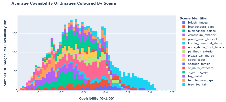
fig = px.histogram(train_df, "mean_covisibility", color="scene", title="<b>Average Covisibility Of Images Coloured By Scene</b>", )
fig.update_layout(
    yaxis_title="<b>Number Of Images Per Covisibility Bin</b>", xaxis_title="<b>Covisibility (0-1.00)</b>",
    legend_title="<b>Scene Identifier</b>",
)
fig.show()

# NOTE: Our intrinsics matrix is a flat string... NOTE: [idx]
#       but when reshaped to 3x3 it will map as follows...
# STRING --> "TL[0] T[1] TR[2] CL[3] C[4] CR[5] BL[6] B[7] BR[8]"
#
# MATRIX BELOW
##############
#            #
#  TL  T  TR #
#  CL  C  CR #
#  BL  B  BR #
#            #
##############
# 
# Therefore we just index into the string and convert to a digit to access certain elements
train_df["fx"] = train_df.camera_intrinsics.apply(lambda x: float(x.split()[0])) # 0 = TL 
train_df["fy"] = train_df.camera_intrinsics.apply(lambda x: float(x.split()[4])) # 4 = C
train_df["x0"] = train_df.camera_intrinsics.apply(lambda x: float(x.split()[2])) # 0 = TR
train_df["y0"] = train_df.camera_intrinsics.apply(lambda x: float(x.split()[5])) # 4 = CR
train_df["s"] = train_df.camera_intrinsics.apply(lambda x: float(x.split()[1])) # 1 = TC

if (train_df["fx"]!=train_df["fy"]).sum()==0:
    print("All fx values (focal length x) are equal to the respective fy values (focal length y)... as expected")
    
if train_df["s"].sum()==0:
    print("All skew values are 0... as expected")

fig = px.histogram(train_df, "x0", title="<b>Principal Point Offset [x<sub>0</sub>] Coloured By Scene</b>", color="scene", log_y=False)
fig.update_layout(
    yaxis_title="<b>Number Of Images Per x<sub>0</sub> Bin</b>", xaxis_title="<b>Principal Point Offset [x<sub>0</sub>]</b>",
    legend_title="<b>Scene Identifier</b>",
)
fig.show()

fig = px.histogram(train_df, "y0", title="<b>Principal Point Offset [y<sub>0</sub>] Coloured By Scene</b>", color="scene", log_y=False)
fig.update_layout(
    yaxis_title="<b>Number Of Images Per y<sub>0</sub> Bin</b>", xaxis_title="<b>Principal Point Offset [y<sub>0</sub>]</b>",
    legend_title="<b>Scene Identifier</b>",
)
fig.show()

# We use "fx" because all "fx" values are equivalent to "fy" values
fig = px.histogram(train_df, "fx", title="<b>Focal Lengths Coloured By Scene</b>", color="scene", log_x=True)
fig.update_layout(
    yaxis_title="<b>Number Of Images Per Focal Length Bin</b>", xaxis_title="<b>Focal Length <i>(log scale)</i></b>",
    legend_title="<b>Scene Identifier</b>",
)
fig.show()

查看相机视角外部

train_df["t_x"] = train_df.translation_vector.apply(lambda x: float(x.split()[0]))
train_df["t_y"] = train_df.translation_vector.apply(lambda x: float(x.split()[1]))
train_df["t_z"] = train_df.translation_vector.apply(lambda x: float(x.split()[2]))

train_df["r1_1"] = train_df.rotation_matrix.apply(lambda x: float(x.split()[0]))
train_df["r2_1"] = train_df.rotation_matrix.apply(lambda x: float(x.split()[1]))
train_df["r3_1"] = train_df.rotation_matrix.apply(lambda x: float(x.split()[2]))
train_df["r1_2"] = train_df.rotation_matrix.apply(lambda x: float(x.split()[3]))
train_df["r2_2"] = train_df.rotation_matrix.apply(lambda x: float(x.split()[4]))
train_df["r3_2"] = train_df.rotation_matrix.apply(lambda x: float(x.split()[5]))
train_df["r1_3"] = train_df.rotation_matrix.apply(lambda x: float(x.split()[6]))
train_df["r2_3"] = train_df.rotation_matrix.apply(lambda x: float(x.split()[7]))
train_df["r3_3"] = train_df.rotation_matrix.apply(lambda x: float(x.split()[8]))

fig = px.histogram(train_df, "t_x", title="<b>Translation Value <sub>x</sub> Coloured By Scene</b>", color="scene", log_y=True)
fig.update_layout(
    yaxis_title="<b>Number Of Images Per Bin <sub>(log-scale)</sub></b>", xaxis_title="<b>Translation Value <sub>x</sub></b>",
    legend_title="<b>Scene Identifier</b>",
)
fig.show()

fig = px.histogram(train_df, "t_y", title="<b>Translation Value <sub>y</sub> Coloured By Scene</b>", color="scene", log_y=True)
fig.update_layout(
    yaxis_title="<b>Number Of Images Per Bin <sub>(log-scale)</sub></b>", xaxis_title="<b>Translation Value <sub>y</sub></b>",
    legend_title="<b>Scene Identifier</b>",
)
fig.show()

fig = px.histogram(train_df, "t_z", title="<b>Translation Value <sub>z</sub> Coloured By Scene</b>", color="scene", log_y=True)
fig.update_layout(
    yaxis_title="<b>Number Of Images Per Bin <sub>(log-scale)</sub></b>", xaxis_title="<b>Translation Value <sub>z</sub></b>",
    legend_title="<b>Scene Identifier</b>",
)
fig.show()


fig = px.histogram(train_df, "r1_1", title="<b>Rotation Value <sub>1,1</sub> Coloured By Scene</b>", color="scene", log_y=True)
fig.update_layout(
    yaxis_title="<b>Number Of Images Per Bin <sub>(log-scale)</sub></b>", xaxis_title="<b>Rotation Value <sub>1,1</sub></b>",
    legend_title="<b>Scene Identifier</b>",
)
fig.show()


fig = px.histogram(train_df, "r2_1", title="<b>Rotation Value <sub>2,1</sub> Coloured By Scene</b>", color="scene", log_y=True)
fig.update_layout(
    yaxis_title="<b>Number Of Images Per Bin <sub>(log-scale)</sub></b>", xaxis_title="<b>Rotation Value <sub>2,1</sub></b>",
    legend_title="<b>Scene Identifier</b>",
)
fig.show()


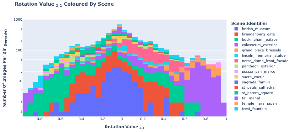
fig = px.histogram(train_df, "r3_1", title="<b>Rotation Value <sub>3,1</sub> Coloured By Scene</b>", color="scene", log_y=True)
fig.update_layout(
    yaxis_title="<b>Number Of Images Per Bin <sub>(log-scale)</sub></b>", xaxis_title="<b>Rotation Value <sub>3,1</sub></b>",
    legend_title="<b>Scene Identifier</b>",
)
fig.show()


fig = px.histogram(train_df, "r1_2", title="<b>Rotation Value <sub>1,2</sub> Coloured By Scene</b>", color="scene", log_y=True)
fig.update_layout(
    yaxis_title="<b>Number Of Images Per Bin <sub>(log-scale)</sub></b>", xaxis_title="<b>Rotation Value <sub>1,2</sub></b>",
    legend_title="<b>Scene Identifier</b>",
)
fig.show()


fig = px.histogram(train_df, "r2_2", title="<b>Rotation Value <sub>2,2</sub> Coloured By Scene</b>", color="scene", log_y=True)
fig.update_layout(
    yaxis_title="<b>Number Of Images Per Bin <sub>(log-scale)</sub></b>", xaxis_title="<b>Rotation Value <sub>2,2</sub></b>",
    legend_title="<b>Scene Identifier</b>",
)
fig.show()


fig = px.histogram(train_df, "r3_2", title="<b>Rotation Value <sub>3,2</sub> Coloured By Scene</b>", color="scene", log_y=True)
fig.update_layout(
    yaxis_title="<b>Number Of Images Per Bin <sub>(log-scale)</sub></b>", xaxis_title="<b>Rotation Value <sub>3,2</sub></b>",
    legend_title="<b>Scene Identifier</b>",
)
fig.show()


fig = px.histogram(train_df, "r1_3", title="<b>Rotation Value <sub>1,3</sub> Coloured By Scene</b>", color="scene", log_y=True)
fig.update_layout(
    yaxis_title="<b>Number Of Images Per Bin <sub>(log-scale)</sub></b>", xaxis_title="<b>Rotation Value <sub>1,3</sub></b>",
    legend_title="<b>Scene Identifier</b>",
)
fig.show()


fig = px.histogram(train_df, "r2_3", title="<b>Rotation Value <sub>2,3</sub> Coloured By Scene</b>", color="scene", log_y=True)
fig.update_layout(
    yaxis_title="<b>Number Of Images Per Bin <sub>(log-scale)</sub></b>", xaxis_title="<b>Rotation Value <sub>2,3</sub></b>",
    legend_title="<b>Scene Identifier</b>",
)
fig.show()

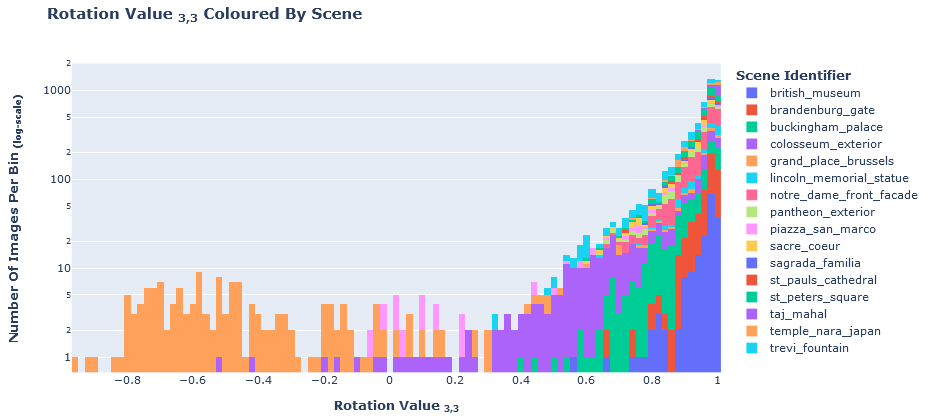
fig = px.histogram(train_df, "r3_3", title="<b>Rotation Value <sub>3,3</sub> Coloured By Scene</b>", color="scene", log_y=True)
fig.update_layout(
    yaxis_title="<b>Number Of Images Per Bin <sub>(log-scale)</sub></b>", xaxis_title="<b>Rotation Value <sub>3,3</sub></b>",
    legend_title="<b>Scene Identifier</b>",
)
fig.show()

看一个带有可识别性和校准信息的示例

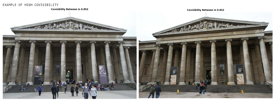
print("\nEXAMPLE OF HIGH COVISIBILITY")
plot_two_paths(
    train_map["british_museum"]["pco_df"]["image_path_1"][0], 
    train_map["british_museum"]["pco_df"]["image_path_2"][0],
    [f"Covisibility Between Is {train_map['british_museum']['pco_df'].covisibility[0]}",
     f"Covisibility Between Is {train_map['british_museum']['pco_df'].covisibility[0]}"]
)

print("\n\n\nIF WE EXAMINE THE CALIBRATION DATAFRAME ROW FOR THE TOP LEFT IMAGE (ID='93658023_4980549800') WE SEE THE FOLLOWING:")
cal_row_from_id = train_map["british_museum"]["cal_df"][train_map["british_museum"]["cal_df"].image_id=="93658023_4980549800"]
for _property in ["camera_intrinsics", "rotation_matrix", "translation_vector"]:
    print(f"\n\n>>>>> {_property.replace('_', ' ').upper()} ARRAY <<<<<\n")
    print(arr_from_str(cal_row_from_id[_property].values[0]))

print("\n\n\nIF WE EXAMINE THE CALIBRATION DATAFRAME ROW FOR THE TOP RIGHT IMAGE (ID='77723525_5227836172') WE SEE THE FOLLOWING:")
cal_row_from_id = train_map["british_museum"]["cal_df"][train_map["british_museum"]["cal_df"].image_id=="77723525_5227836172"]
for _property in ["camera_intrinsics", "rotation_matrix", "translation_vector"]:
    print(f"\n\n>>>>> {_property.replace('_', ' ').upper()} ARRAY <<<<<\n")
    print(arr_from_str(cal_row_from_id[_property].values[0]))

    
print("\n\n\n\nEXAMPLE OF NO COVISIBILITY")
plot_two_paths(
    train_map["british_museum"]["pco_df"]["image_path_1"][15395],
    train_map["british_museum"]["pco_df"]["image_path_2"][15395],
    [f"Covisibility Between Is {train_map['british_museum']['pco_df'].covisibility[15395]}",
     f"Covisibility Between Is {train_map['british_museum']['pco_df'].covisibility[15395]}"]
)

print("\n\n\nIF WE EXAMINE THE CALIBRATION DATAFRAME ROW FOR THE TOP LEFT IMAGE (ID='66757775_3535589713') WE SEE THE FOLLOWING:")
cal_row_from_id = train_map["british_museum"]["cal_df"][train_map["british_museum"]["cal_df"].image_id=="66757775_3535589713"]
for _property in ["camera_intrinsics", "rotation_matrix", "translation_vector"]:
    print(f"\n\n>>>>> {_property.replace('_', ' ').upper()} ARRAY <<<<<\n")
    print(arr_from_str(cal_row_from_id[_property].values[0]))

print("\n\n\nIF WE EXAMINE THE CALIBRATION DATAFRAME ROW FOR THE TOP RIGHT IMAGE (ID='66747696_4734591579') WE SEE THE FOLLOWING:")
cal_row_from_id = train_map["british_museum"]["cal_df"][train_map["british_museum"]["cal_df"].image_id=="66747696_4734591579"]
for _property in ["camera_intrinsics", "rotation_matrix", "translation_vector"]:
    print(f"\n\n>>>>> {_property.replace('_', ' ').upper()} ARRAY <<<<<\n")
    print(arr_from_str(cal_row_from_id[_property].values[0]))

4.6 绘制每个场景并具有可识别性

for _s in TRAIN_SCENES:
    print(f"\n\n\nRANDOM PLOT FOR {_s} LOCATION SCENE")
    pco_random_plot(train_map[_s]["pco_df"])

4.7 将一个图像的关键点映射到另一个图像（基本筛选）

# Step 1 - 选择图像对并显示
DEMO_ROW = train_map["taj_mahal"]["pco_df"].iloc[850]
DEMO_IMG_ID_1 = DEMO_ROW.image_id_1
DEMO_IMG_ID_2 = DEMO_ROW.image_id_2
DEMO_PATH_1 = DEMO_ROW.image_path_1
DEMO_PATH_2 = DEMO_ROW.image_path_2

demo_img_1 = cv2.imread(DEMO_PATH_1)[..., ::-1]
demo_img_2 = cv2.imread(DEMO_PATH_2)[..., ::-1]

# FM= Fundamental Matrix
DEMO_F = arr_from_str(DEMO_ROW.fundamental_matrix)

plot_two_paths(DEMO_PATH_1, DEMO_PATH_2, _titles=[f"IMAGE ID 1: {DEMO_IMG_ID_1}", f"IMAGE ID 2: {DEMO_IMG_ID_2}"])

##################################################################
# Step 2 - 使用 SIFT检测图像中的关键点 #
##################################################################
n_feat = 1_000


contrast_thresh = -10_000
edge_thresh = -10_000

sift_detector = cv2.SIFT_create(n_feat, contrastThreshold=contrast_thresh, edgeThreshold=edge_thresh)

keypoints_1, descriptors_1 = extract_sift_features(demo_img_1, sift_detector, n_feat)
keypoints_2, descriptors_2 = extract_sift_features(demo_img_2, sift_detector, n_feat)

# Each local feature contains a keypoint (xy, possibly scale, possibly orientation) and a description vector (128-dimensional for SIFT).
#   DRAW_RICH_KEYPOINTS Description: 
#        --> For each keypoint the circle around keypoint with keypoint size and orientation will be drawn.
image_with_keypoints_1 = cv2.drawKeypoints(demo_img_1, keypoints_1, outImage=None, flags=cv2.DRAW_MATCHES_FLAGS_DRAW_RICH_KEYPOINTS)
plt.figure(figsize=(20, 15))
plt.imshow(image_with_keypoints_1)
plt.axis(False)
plt.show()

image_with_keypoints_2 = cv2.drawKeypoints(demo_img_2, keypoints_2, outImage=None, flags=cv2.DRAW_MATCHES_FLAGS_DRAW_RICH_KEYPOINTS)
plt.figure(figsize=(20, 15))
plt.imshow(image_with_keypoints_2)
plt.axis(False)
plt.show()

###################################################################################
# Step 3 - 匹配从图像 1 到图像 2 的关键点#
###################################################################################

bfm = cv2.BFMatcher(cv2.NORM_L2, crossCheck=True)

# Compute matches and reduce to [query|train] indexors
cv_matches = bfm.match(descriptors_1, descriptors_2)
matches_before = np.array([[m.queryIdx, m.trainIdx] for m in cv_matches])

# Convert keypoints and matches to something more human-readable.
kp_1_pos = np.array([kp.pt for kp in keypoints_1])
kp_2_pos = np.array([kp.pt for kp in keypoints_2])
kp_matches = np.array([[m.queryIdx, m.trainIdx] for m in cv_matches])

img_matches_before = draw_cv_matches(demo_img_1, demo_img_2, kp_1_pos, kp_2_pos, matches_before)
plt.figure(figsize=(20, 15))
plt.title('Matches BEFORE RANSAC', fontweight="bold")
plt.imshow(img_matches_before)
plt.axis(False)
plt.show()


F, inlier_mask = cv2.findFundamentalMat(kp_1_pos[matches_before[:, 0]], kp_2_pos[matches_before[:, 1]], 
                                        cv2.USAC_MAGSAC, ransacReprojThreshold=0.25, 
                                        confidence=0.99999, maxIters=10000)
#########################################################################################################

matches_after = np.array([match for match, is_inlier in zip(matches_before, inlier_mask) if is_inlier])
img_matches_after = draw_cv_matches(demo_img_1, demo_img_2, kp_1_pos, kp_2_pos, matches_after)
plt.figure(figsize=(20, 15))
plt.title('Matches AFTER RANSAC', fontweight="bold")
plt.imshow(img_matches_after)
plt.axis(False)
plt.show()

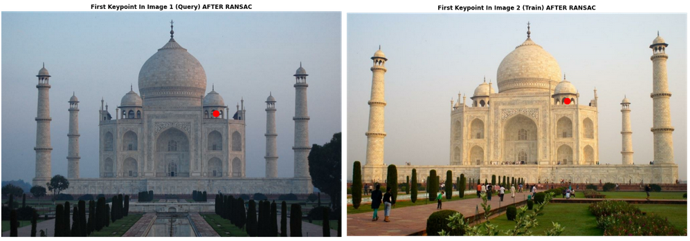
# CHECK THE FIRST KEYPOINT
match_query_kp_position_1 = keypoints_1[matches_after[0][0]].pt
match_query_kp_position_1 = (int(round(match_query_kp_position_1[0])), 
                             int(round(match_query_kp_position_1[1])))
match_train_kp_position_1 = keypoints_2[matches_after[0][1]].pt
match_train_kp_position_1 = (int(round(match_train_kp_position_1[0])), 
                             int(round(match_train_kp_position_1[1])))
_tmp_1 = cv2.circle(demo_img_1.copy(), match_query_kp_position_1, 10, (255,0,0), -1)
_tmp_2 = cv2.circle(demo_img_2.copy(), match_train_kp_position_1, 10, (255,0,0), -1)

plt.figure(figsize=(20,10))
plt.subplot(1,2,1)
plt.title("First Keypoint In Image 1 (Query) AFTER RANSAC", fontweight="bold")
plt.axis(False)
plt.imshow(_tmp_1)

plt.subplot(1,2,2)
plt.title("First Keypoint In Image 2 (Train) AFTER RANSAC", fontweight="bold")
plt.axis(False)
plt.imshow(_tmp_2)

plt.tight_layout()
plt.show()

# CHECK THE SECOND KEYPOINT
match_query_kp_position_2 = keypoints_1[matches_after[1][0]].pt
match_query_kp_position_2 = (int(round(match_query_kp_position_2[0])), 
                             int(round(match_query_kp_position_2[1])))
match_train_kp_position_2 = keypoints_2[matches_after[1][1]].pt
match_train_kp_position_2 = (int(round(match_train_kp_position_2[0])), 
                             int(round(match_train_kp_position_2[1])))

_tmp_1 = cv2.circle(_tmp_1, match_query_kp_position_2, 10, (0,255,0), -1)
_tmp_2 = cv2.circle(_tmp_2, match_train_kp_position_2, 10, (0,255,0), -1)

plt.figure(figsize=(20,10))
plt.subplot(1,2,1)
plt.title("Second Keypoint In Image 1 (Query) AFTER RANSAC", fontweight="bold")
plt.axis(False)
plt.imshow(_tmp_1)

plt.subplot(1,2,2)
plt.title("Second Keypoint In Image 2 (Train) AFTER RANSAC", fontweight="bold")
plt.axis(False)
plt.imshow(_tmp_2)
plt.tight_layout()
plt.show()

# CHECK THE THIRD KEYPOINT
match_query_kp_position_3 = keypoints_1[matches_after[2][0]].pt
match_query_kp_position_3 = (int(round(match_query_kp_position_3[0])), 
                             int(round(match_query_kp_position_3[1])))
match_train_kp_position_3 = keypoints_2[matches_after[2][1]].pt
match_train_kp_position_3 = (int(round(match_train_kp_position_3[0])), 
                             int(round(match_train_kp_position_3[1])))

_tmp_1 = cv2.circle(_tmp_1, match_query_kp_position_3, 10, (0,0,255), -1)
_tmp_2 = cv2.circle(_tmp_2, match_train_kp_position_3, 10, (0,0,255), -1)

plt.figure(figsize=(20,10))
plt.subplot(1,2,1)
plt.title("Third Keypoint In Image 1 (Query) AFTER RANSAC", fontweight="bold")
plt.axis(False)
plt.imshow(_tmp_1)

plt.subplot(1,2,2)
plt.title("Third Keypoint In Image 2 (Train) AFTER RANSAC", fontweight="bold")
plt.axis(False)
plt.imshow(_tmp_2)
plt.tight_layout()
plt.show()

浩波的笔记

关注

1
点赞
踩
4

收藏

觉得还不错? 一键收藏
0
评论
[数据分析实践]-Image Matching-2DTo3D-1

让机器学习使用互联网上免费提供的大量非结构化图像集合，来帮助更好地捕捉世界的丰富性，这个想法怎么样？从图像重建 3D 对象和建筑物的过程称为运动结构 (SfM)。
复制链接

扫一扫