北京二手房数据分析

目的

本案例得目标主要对数据集中的特征进行量化分析，并且通过图形可视化进行展示出来。项目数据来源于链家北京二手房数据。

数据预处理

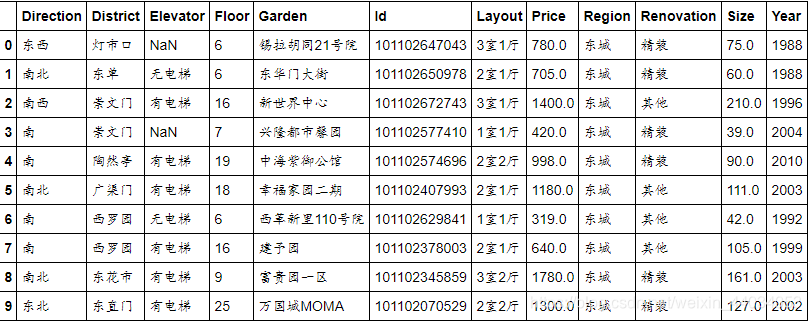
首先导入分析过程中可能运用到的函数包，并读取显示前10行数据。

import pandas as pd
import numpy as np
import matplotlib.pyplot as plt
import matplotlib as mpl
import seaborn as sns
from IPython.display import display
%matplotlib inline

lianjia_df=pd.read_csv('lianjia.csv')
lianjia_df.head(10)

前10行数据结果显示如下所示

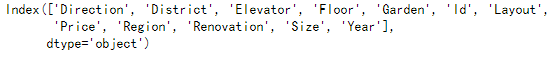
然后对数据的基本信息进行查看

lianjia_df.index
lianjia_df.columns
lianjia_df.info()

以上三条代码分别显示如下



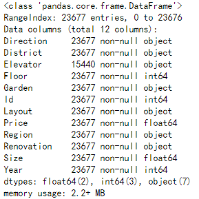
再对数据进行描述性统计

lianjia_df.describe()

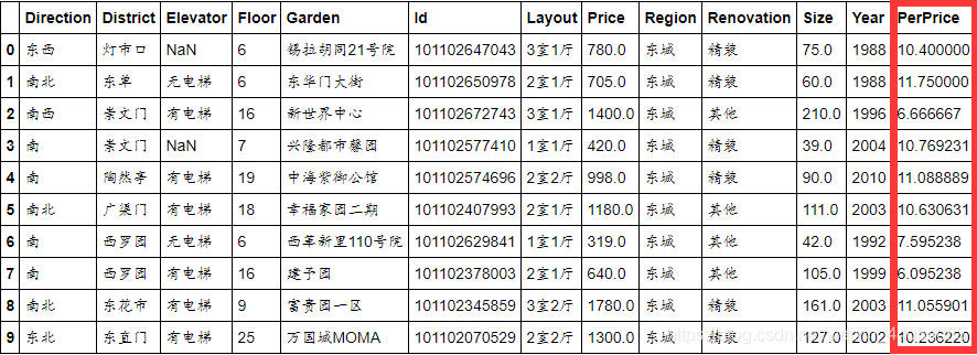
新建特征PerPrice，其值等于房价除以面积，并显示前10行数据

df=lianjia_df.copy()
df['PerPrice']=lianjia_df['Price']/lianjia_df['Size']
df[:10]

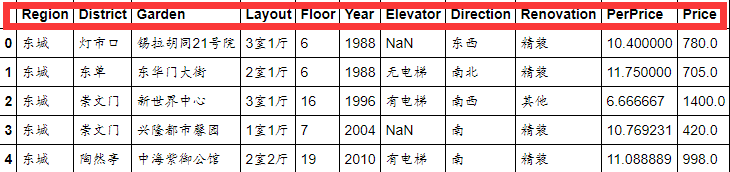
对数据的属性重新排列，并将一些无用的属性删除，最后显示前5行数据，代码及结果显示如下

columns=['Region','District','Garden','Layout','Floor','Year','Elevator','Direction','Renovation','PerPrice','Price']
df=pd.DataFrame(df,columns=columns)
df.head()

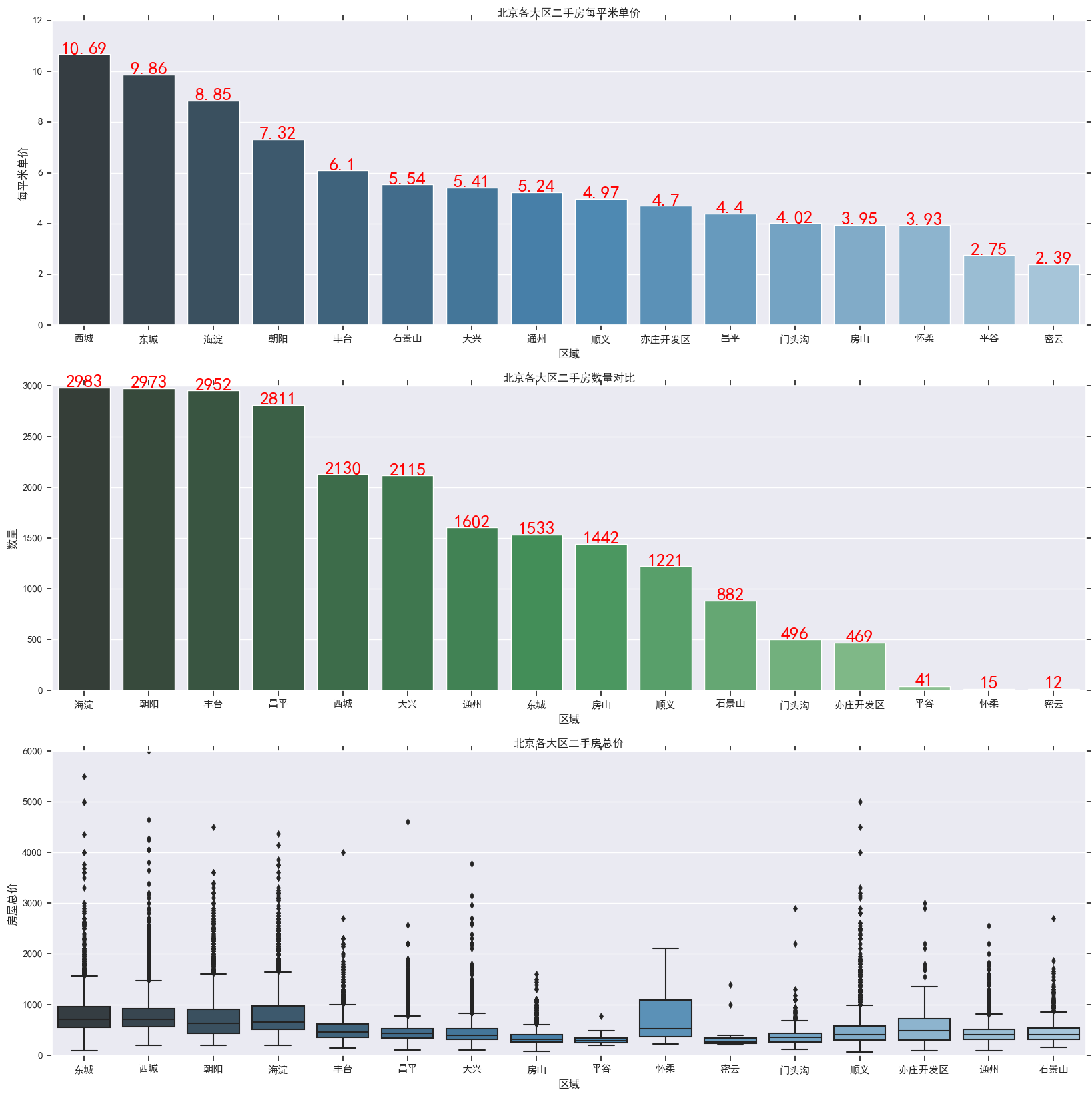
对各个地区的价格进行分析

首先按照地区对价格进行分组，其次按照地区对PerPrice进行分组，然后利用柱形图与箱型图进行可视化

df_house_count=df.groupby('Region')['Price'].count().sort_values(ascending=False)
df_house_count=df_house_count.to_frame().reset_index()

df_house_mean=df.groupby('Region')['PerPrice'].mean().sort_values(ascending=False)
df_house_mean=df_house_mean.to_frame().reset_index()

f,[ax1,ax2,ax3]=plt.subplots(3,1,figsize=(20,20))
sns.set(font='SimHei')
m=sns.barplot(x='Region',y='PerPrice',palette='Blues_d',data=df_house_mean,ax=ax1)

"""在柱形图上添加数字"""
for index,row in df_house_mean.iterrows(): 
    m.text(row.name,row.PerPrice,round(row.PerPrice,2),ha='center',color='red',fontsize=20)
    
ax1.set_title('北京各大区二手房每平米单价')
ax1.set_xlabel('区域')
ax1.set_ylabel('每平米单价')

b=sns.barplot(x='Region',y='Price',palette='Greens_d',data=df_house_count,ax=ax2)

for index,row in df_house_count.iterrows():
    b.text(row.name,row.Price,round(row.Price,2),ha='center',color='red',fontsize=20)
    
ax2.set_title('北京各大区二手房数量对比')
ax2.set_xlabel('区域')
ax2.set_ylabel('数量')

sns.boxplot(x='Region',y='Price',palette='Blues_d',data=df,ax=ax3)
ax3.set_title('北京各大区二手房总价')
ax3.set_xlabel('区域')
ax3.set_ylabel('房屋总价')

plt.show()

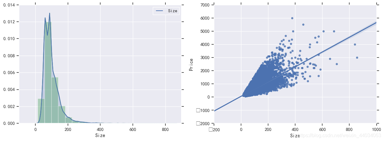
Size特征分析

f,[ax1,ax2]=plt.subplots(1,2,figsize=(15,5))
sns.distplot(df["Size"],bins=20,ax=ax1,color='g')
sns.kdeplot(df.Size,shade=1,ax=ax1)  #kdeplot()核密度估计图：估计未知的密度函数，属于非参数检验方法之一
sns.regplot(x='Size',y='Price',data=df,ax=ax2)
plt.show()

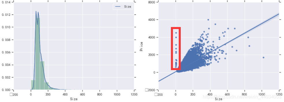
在右图中，出现一些离散值，需要将其去除

df=df.loc[(df.Size>10)&(df.Size<1000)]

f,[ax1,ax2]=plt.subplots(1,2,figsize=(15,5))
sns.distplot(df["Size"],bins=20,ax=ax1,color='g')
sns.kdeplot(df.Size,shade=1,ax=ax1)  #kdeplot()核密度估计图：估计未知的密度函数，属于非参数检验方法之一
sns.regplot(x='Size',y='Price',data=df,ax=ax2)
plt.show()

处理后的可视化如上图所示

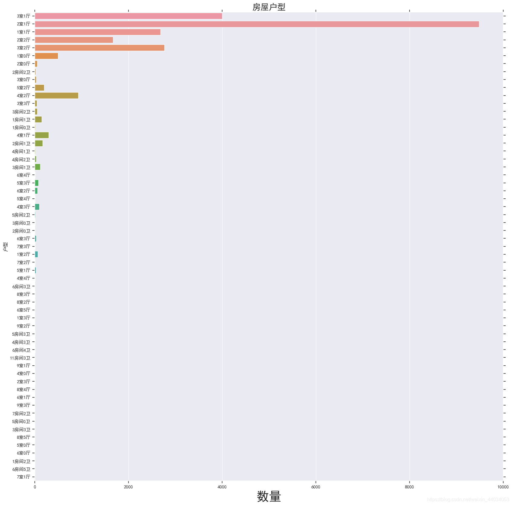
户型分析

f,ax1=plt.subplots(figsize=(20,20))
sns.countplot(y='Layout',data=df,ax=ax1)
ax1.set_title('房屋户型',fontsize=20)
ax1.set_xlabel('数量',fontsize=30)
ax1.set_ylabel('户型')
plt.show()

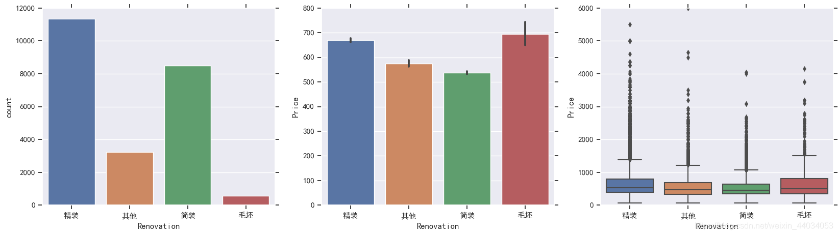
Renovation特征分析

df["Renovation"]=df.loc[(df.Renovation!='南北'),'Renovation']

f,[ax1,ax2,ax3]=plt.subplots(1,3,figsize=(20,5))
sns.countplot(df.Renovation,ax=ax1)
sns.barplot(x='Renovation',y='Price',data=df,ax=ax2)
sns.boxplot(x='Renovation',y='Price',data=df,ax=ax3)
plt.show()

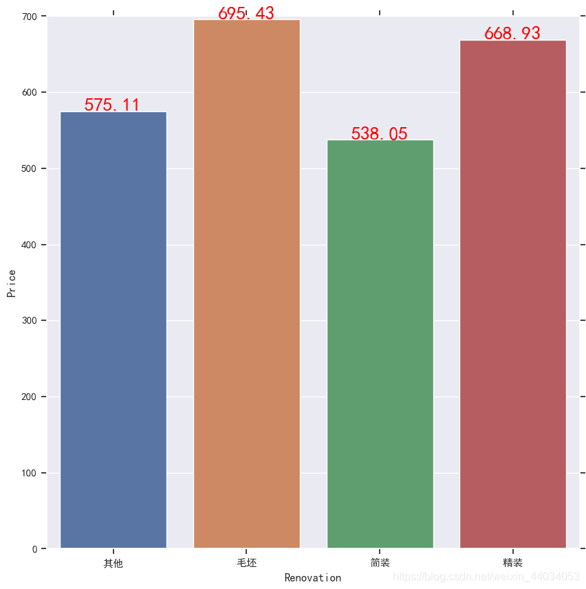
对第二个图进行改进后如下代码和结果显示

df4=df.groupby('Renovation')['Price'].mean().to_frame().reset_index()
f,ax2=plt.subplots(figsize=(10,10))
n=sns.barplot(x='Renovation',y='Price',data=df4,ax=ax2)
for ind,row in df4.iterrows():
    n.text(row.name,row.Price,round(row.Price,2),ha='center',color='red',fontsize=20)
plt.show()

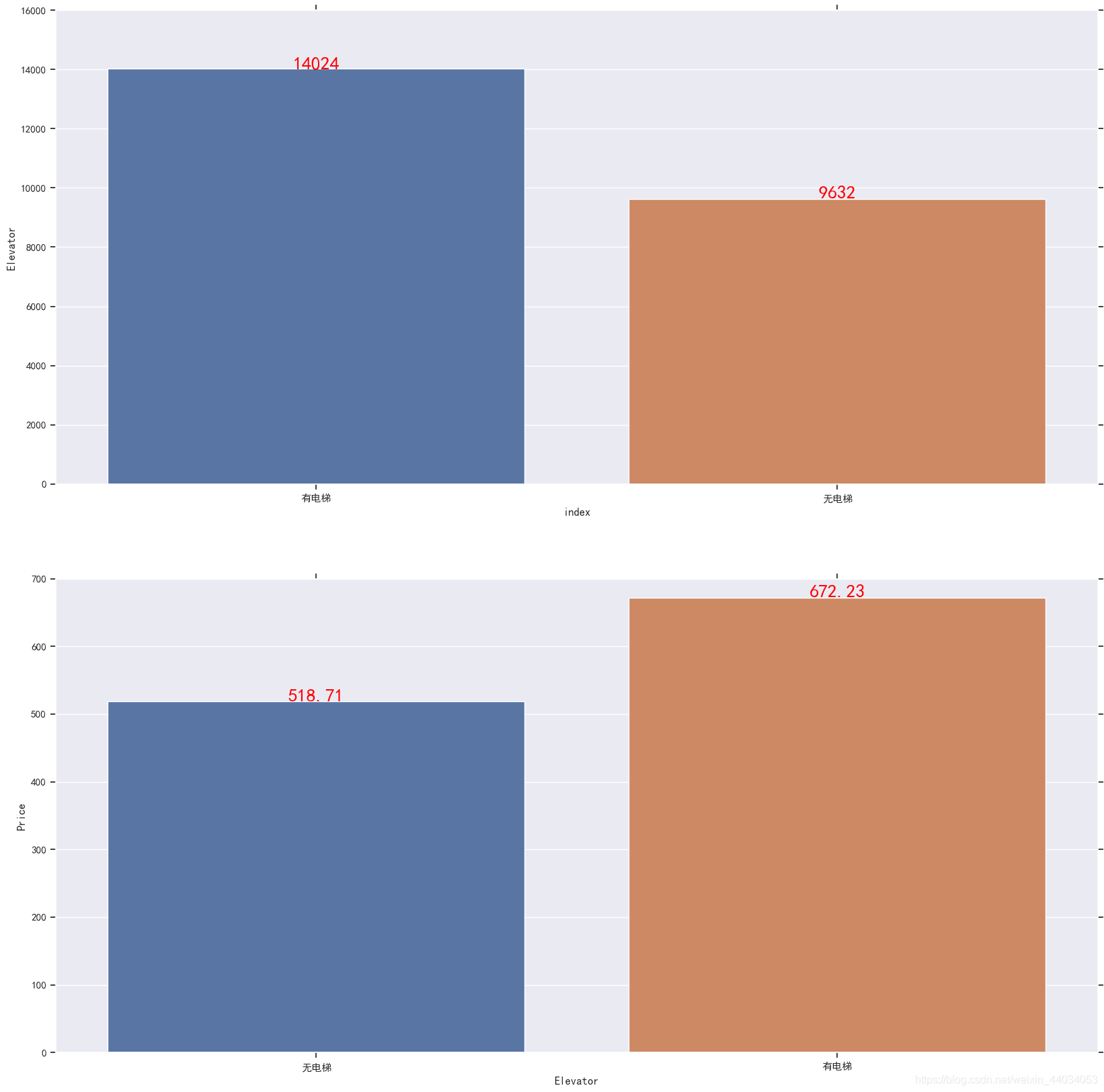
Elevator特征分析

df.loc[(df.Floor<=6)&(df.Elevator.isnull()),'Elevator']='无电梯'
df.loc[(df.Floor>6)&(df.Elevator.isnull()),'Elevator']='有电梯'
df5=df.Elevator.value_counts().to_frame().reset_index()

df6=df.groupby('Elevator')['Price'].mean().to_frame().reset_index()

f,[ax1,ax2]=plt.subplots(2,1,figsize=(20,20))
h=sns.barplot(x='index',y='Elevator',data=df5,ax=ax1)
for inde,row in df5.iterrows():
    h.text(row.name,row.Elevator,round(row.Elevator,2),ha='center',color='red',fontsize=20)

i=sns.barplot(x='Elevator',y='Price',data=df6,ax=ax2)
for inde,row in df6.iterrows():
    i.text(row.name,row.Price,round(row.Price,2),ha='center',color='red',fontsize=20)
plt.show()

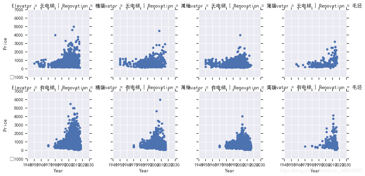
Year特征分析

y=sns.FacetGrid(df,row='Elevator',col='Renovation')
y.map(plt.scatter,'Year','Price')

Floor特征分析

f,ax1=plt.subplots(figsize=(20,5))
r=sns.countplot(x='Floor',data=df,ax=ax1)
plt.show()